Reverse Modelling of an Emission Spectrum
Update: June 1/2021, Hajime Kawahara
import pandas as pd
import numpy as np
import matplotlib.pyplot as plt
import jax.numpy as jnp
Here, we use the mock spectrum generated by “Forward Modelling of an Emission Spectrum”.
dat=pd.read_csv("spectrum.txt",delimiter=",",names=("wav","flux"))
We add Gaussian noise to data. nusd is the observing wavenumber grid.
wavd=dat["wav"].values
flux=dat["flux"].values
nusd=jnp.array(1.e8/wavd[::-1])
sigmain=0.05
norm=40000
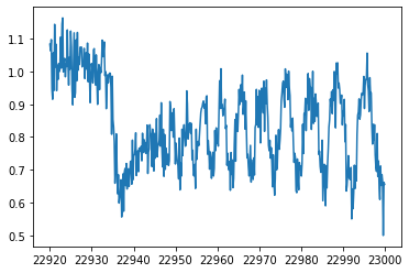
nflux=flux/norm+np.random.normal(0,sigmain,len(wavd))
plt.plot(wavd[::-1],nflux)

from exojax.spec.lpf import xsmatrix
from exojax.spec.exomol import gamma_exomol
from exojax.spec.hitran import SijT, doppler_sigma, gamma_natural, gamma_hitran
from exojax.spec.hitrancia import read_cia, logacia
from exojax.spec.rtransfer import rtrun, dtauM, dtauCIA, nugrid
from exojax.spec import planck, response
from exojax.spec.lpf import xsvector
from exojax.spec import molinfo
from exojax.utils.constants import RJ, pc, Rs, c
The model is almost same as the forward modeling, but we will infer here Rp, RV, MMR_CO, T0, alpha, and Vsini.
from exojax.spec import rtransfer as rt
NP=100
Parr, dParr, k=rt.pressure_layer(NP=NP)
Nx=1500
nus,wav,res=nugrid(np.min(wavd)-5.0,np.max(wavd)+5.0,Nx,unit="AA")

R=100000.
beta=c/(2.0*np.sqrt(2.0*np.log(2.0))*R)

molmassCO=molinfo.molmass("CO")
mmw=2.33 #mean molecular weight
mmrH2=0.74
molmassH2=molinfo.molmass("H2")
vmrH2=(mmrH2*mmw/molmassH2) #VMR

Mp = 33.2 #fixing mass...
Loading the molecular database of CO and the CIA
from exojax.spec import moldb, contdb
mdbCO=moldb.MdbExomol('.database/CO/12C-16O/Li2015',nus,crit=1.e-46)
cdbH2H2=contdb.CdbCIA('.database/H2-H2_2011.cia',nus)
Background atmosphere:  H2
Reading transition file
Broadening code level= a0
H2-H2
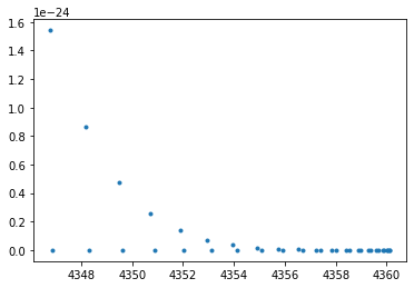
We have only 39 CO lines.
plt.plot(mdbCO.nu_lines,mdbCO.Sij0,".")

Again, numatrix should be precomputed prior to HMC-NUTS.
from exojax.spec import make_numatrix0
numatrix_CO=make_numatrix0(nus,mdbCO.nu_lines)
#reference pressure for a T-P model
Pref=1.0 #bar
ONEARR=np.ones_like(Parr)
import jax.numpy as jnp
from jax import random
from jax import vmap, jit

import numpyro.distributions as dist
import numpyro
from numpyro.infer import MCMC, NUTS
from numpyro.infer import Predictive
from numpyro.diagnostics import hpdi
Now we write the model, which is used in HMC-NUTS.
def model_c(nu1,y1):
    Rp = numpyro.sample('Rp', dist.Uniform(0.5,1.2))
    RV = numpyro.sample('RV', dist.Uniform(5.0,15.0))
    MMR_CO = numpyro.sample('MMR_CO', dist.Uniform(0.0,0.01))
    T0 = numpyro.sample('T0', dist.Uniform(1000.0,1500.0))
    alpha=numpyro.sample('alpha', dist.Uniform(0.05,0.2))
    vsini = numpyro.sample('vsini', dist.Uniform(15.0,25.0))
    g=2478.57730044555*Mp/Rp**2 #gravity
    u1=0.0
    u2=0.0
    #T-P model//
    Tarr = T0*(Parr/Pref)**alpha

    #line computation CO
    qt_CO=vmap(mdbCO.qr_interp)(Tarr)

    def obyo(y,tag,nusd,nus,numatrix_CO,mdbCO,cdbH2H2):
        #CO
        SijM_CO=jit(vmap(SijT,(0,None,None,None,0)))\
            (Tarr,mdbCO.logsij0,mdbCO.dev_nu_lines,mdbCO.elower,qt_CO)
        gammaLMP_CO = jit(vmap(gamma_exomol,(0,0,None,None)))\
            (Parr,Tarr,mdbCO.n_Texp,mdbCO.alpha_ref)
        gammaLMN_CO=gamma_natural(mdbCO.A)
        gammaLM_CO=gammaLMP_CO+gammaLMN_CO[None,:]

        sigmaDM_CO=jit(vmap(doppler_sigma,(None,0,None)))\
            (mdbCO.dev_nu_lines,Tarr,molmassCO)
        xsm_CO=xsmatrix(numatrix_CO,sigmaDM_CO,gammaLM_CO,SijM_CO)
        dtaumCO=dtauM(dParr,xsm_CO,MMR_CO*ONEARR,molmassCO,g)
        #CIA
        dtaucH2H2=dtauCIA(nus,Tarr,Parr,dParr,vmrH2,vmrH2,\
                          mmw,g,cdbH2H2.nucia,cdbH2H2.tcia,cdbH2H2.logac)
        dtau=dtaumCO+dtaucH2H2
        sourcef = planck.piBarr(Tarr,nus)
        F0=rtrun(dtau,sourcef)/norm

        Frot=response.rigidrot(nus,F0,vsini,u1,u2)
        mu=response.ipgauss_sampling(nusd,nus,Frot,beta,RV)
        numpyro.sample(tag, dist.Normal(mu, sigmain), obs=y)

    obyo(y1,"y1",nu1,nus,numatrix_CO,mdbCO,cdbH2H2)
Run a HMC-NUTS. It took ~37min using my gaming laptop (razer blade 15, GTX 1080 Max-Q). Here, the number of warmup sampling is only 300, and that of real sampling is only 600, because the time when the draft on arxiv will be released is very soon and I am writing this eating breakfast (in June 1st 2021 morning in JST!). Note that we here use forward mode (forward differentiation) by ‘forward_mode_differentiation=True’ in NUTS. Since ExoJAX v1.1, we can also use the reverse mode ‘forward_mode_differentiation=False’ in NUTS.
rng_key = random.PRNGKey(0)
rng_key, rng_key_ = random.split(rng_key)
num_warmup, num_samples = 300, 600
kernel = NUTS(model_c,forward_mode_differentiation=True)
mcmc = MCMC(kernel, num_warmup, num_samples)
mcmc.run(rng_key_, nu1=nusd, y1=nflux)
sample: 100%|██████████| 900/900 [37:05<00:00, 2.53s/it, 127 steps of size 3.88e-02. acc. prob=0.90]
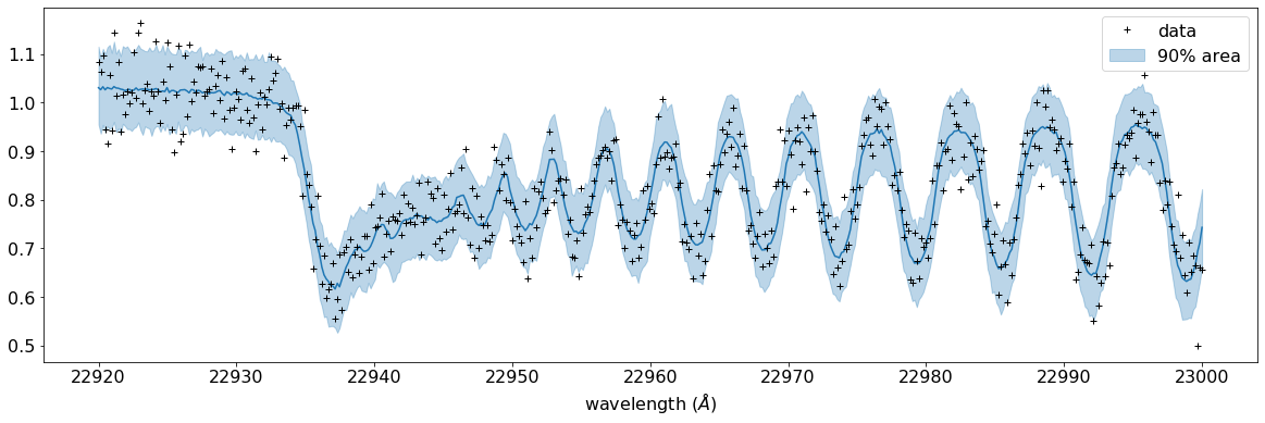
Plotting a prediction and 90% area with the data… looks good.
posterior_sample = mcmc.get_samples()
pred = Predictive(model_c,posterior_sample,return_sites=["y1"])
predictions = pred(rng_key_,nu1=nusd,y1=None)
median_mu1 = jnp.median(predictions["y1"],axis=0)
hpdi_mu1 = hpdi(predictions["y1"], 0.9)
fig, ax = plt.subplots(nrows=1, ncols=1, figsize=(20,6.0))
ax.plot(wavd[::-1],median_mu1,color="C0")
ax.plot(wavd[::-1],nflux,"+",color="black",label="data")
ax.fill_between(wavd[::-1], hpdi_mu1[0], hpdi_mu1[1], alpha=0.3, interpolate=True,color="C0",label="90% area")
plt.xlabel("wavelength ($\AA$)",fontsize=16)
plt.legend(fontsize=16)
plt.tick_params(labelsize=16)

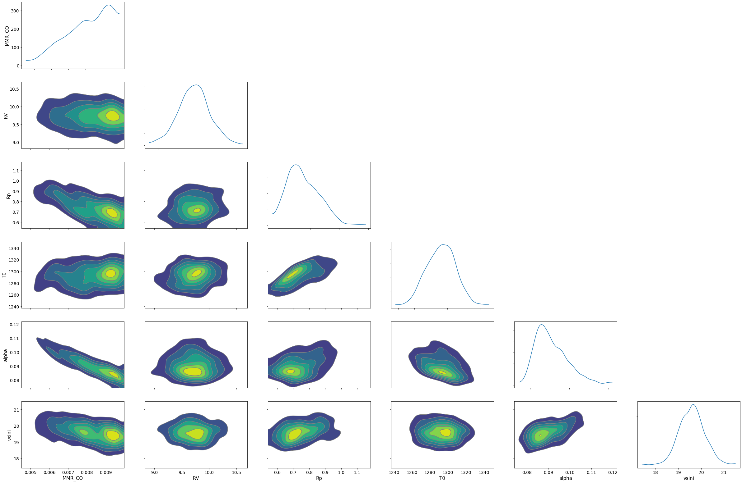
Arviz is useful to visualize the corner plot. For the above reasons, I haven’t been checkingthe results properly. Ah, the range of prior looks too narrow for some parameters. But I have to take the boy to kindergarten soon. Try to change the priors and to run a HMC-NUTS again, with maybe longer chains! The rest is up to you.
import arviz
pararr=["Rp","T0","alpha","MMR_CO","vsini","RV"]
arviz.plot_pair(arviz.from_numpyro(mcmc),kind='kde',divergences=False,marginals=True)
plt.show()

For fitting to the real spectrum, we may need a more well-considered model and a better GPU, such as V100 or A100. Read the next section “🐱 Bayes Inference of a Real Spectrum of Luhman 16A (Direct LPF)” in detail.