Rigid Stellar Rotation and Gaussian Convolution¶

Here, we apply a rigid stellar rotation model to a mock spectrum.

import numpy as np
from exojax.spec.rtransfer import nugrid
from exojax.spec import response

Setting a wavenumber grid as

nus,wav,res=nugrid(23000,23100,2000,unit="AA")

and a mock spectrum, which exhibits a sharp dip in the center.

#1 - delta function like
F=np.ones_like(nus)
F[1000]=0.0

Assuming Vsini=100km/s

vsini=100.0 #km/s

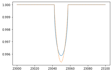
response.rigidrot convolves a rigid (solid-body) rotation kernel to F. We can also take consideration limb darkening with the coefficients (u1, u2).

import matplotlib.pyplot as plt
plt.plot(wav,response.rigidrot(nus,F,vsini,u1=0.0,u2=0.0),lw=1)
plt.plot(wav,response.rigidrot(nus,F,vsini,u1=0.6,u2=0.4),lw=1,ls="dashed")
plt.show()

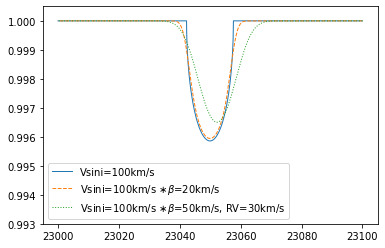
Gaussian covolution and velocity shift can be involved using response.ipgauss_sampling

Frot=response.rigidrot(nus,F,vsini,u1=0.0,u2=0.0)
Fx=response.ipgauss_sampling(nus,nus,Frot,20.0,0.0)
Fxx=response.ipgauss_sampling(nus,nus,Frot,50.0,30.0)

plt.plot(wav[::-1],Frot,lw=1,label="Vsini=100km/s")
plt.plot(wav[::-1],Fx,lw=1,ls="dashed",label="Vsini=100km/s $\\ast \\beta$=20km/s")
plt.plot(wav[::-1],Fxx,lw=1,ls="dotted",label="Vsini=100km/s $\\ast \\beta$=50km/s, RV=30km/s")
plt.legend(loc="lower left")
plt.ylim(0.993,1.0005)
plt.show()

The summation is conserved.

print(np.sum(F))
print(np.sum(response.rigidrot(nus,F,vsini,u1=0.6,u2=0.4)))
print(np.sum(response.rigidrot(nus,F,vsini,u1=0.0,u2=0.0)))
print(np.sum(Fx))