Forward Modelling of an Emission Spectrum

Update: June 1/2021, Hajime Kawahara

First, we set a planet atmosphere model as

\(T = T_0 P^{0.1}\)

in the unit of K and bar for T and P.

from exojax.spec import rtransfer as rt

#ATMOSPHERE
NP=100
T0=1300.0 #K
Parr, dParr, k=rt.pressure_layer(NP=NP)
Tarr = T0*(Parr)**0.1

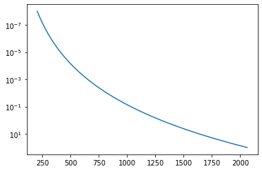
A T-P profile we assume is like that.

import matplotlib.pyplot as plt
plt.plot(Tarr,Parr)
plt.yscale("log")
plt.gca().invert_yaxis()
plt.show()

We set a wavenumber grid using nugrid. Note that nugrid sets the wavenumber grid evenly spaced in log space. We need such the grid to apply an instrumental and rotational responses to a raw spectrum.

from exojax.spec.rtransfer import nugrid
nus,wav,res=nugrid(22920,23000,1000,unit="AA")

Loading a molecular database of CO and CIA (H2-H2)…

from exojax.spec import moldb, contdb
mdbCO=moldb.MdbExomol('.database/CO/12C-16O/Li2015',nus)
cdbH2H2=contdb.CdbCIA('.database/H2-H2_2011.cia',nus)

Background atmosphere:  H2
Reading transition file
Broadening code level= a0
default broadening parameters are used for  71  J lower states in  152  states
H2-H2

The molecular mass is given as

from exojax.spec import molinfo
molmassCO=molinfo.molmass("CO")

Computing the normalized partition function \(q_t = Q(T)/Q(T_\mathrm{ref})\) …

from jax import vmap
qt=vmap(mdbCO.qr_interp)(Tarr)

Computing the gamma parameters for the pressure and natural broadenings…

from jax import jit
from exojax.spec.exomol import gamma_exomol
from exojax.spec import gamma_natural

gammaLMP = jit(vmap(gamma_exomol,(0,0,None,None)))\
        (Parr,Tarr,mdbCO.n_Texp,mdbCO.alpha_ref)
gammaLMN=gamma_natural(mdbCO.A)
gammaLM=gammaLMP+gammaLMN[None,:]

The sigma for the Doppler broadening is given as

from exojax.spec import doppler_sigma
sigmaDM=jit(vmap(doppler_sigma,(None,0,None)))\
        (mdbCO.nu_lines,Tarr,molmassCO)

We also compute the line strength matrix as

from exojax.spec import SijT
SijM=jit(vmap(SijT,(0,None,None,None,0)))\
    (Tarr,mdbCO.logsij0,mdbCO.nu_lines,mdbCO.elower,qt)

nu matrix is a matrix that contains wavenumber grids around line centers.

from exojax.spec import make_numatrix0
numatrix=make_numatrix0(nus,mdbCO.nu_lines)

Providing numatrix, thermal broadening, gamma, and line strength, we can compute cross section.

from exojax.spec.lpf import xsmatrix
xsm=xsmatrix(numatrix,sigmaDM,gammaLM,SijM)

xsmatrix has the shape of (# of layers, # of nu grid)

import numpy as np
np.shape(xsm)

(100, 1000)

So, this is a visualization of xsmatrix.

import numpy as np
plt.imshow(xsm,cmap="afmhot")
plt.show()

We compute delta tau (tau in layers) for CO,

from exojax.spec.rtransfer import dtauM
g=1.e5 #gravity cm/s2
MMR=0.01 #mass mixing ratio
dtaum=dtauM(dParr,xsm,MMR*np.ones_like(Tarr),molmassCO,g)

and delta tau for CIA

from exojax.spec.rtransfer import dtauCIA
mmw=2.33 #mean molecular weight
mmrH2=0.74
molmassH2=molinfo.molmass("H2")
vmrH2=(mmrH2*mmw/molmassH2) #VMR
dtaucH2H2=dtauCIA(nus,Tarr,Parr,dParr,vmrH2,vmrH2,\
            mmw,g,cdbH2H2.nucia,cdbH2H2.tcia,cdbH2H2.logac)

The total delta tau is a summation of them

dtau=dtaum+dtaucH2H2

We can plot a contribution function using exojax.plot.atmplot as

from exojax.plot.atmplot import plotcf
plotcf(nus,dtau,Tarr,Parr,dParr)
plt.show()

We perform a radiative transfer. Here, the source function is the Planck function (multiplied by pi).

from exojax.spec import planck
from exojax.spec.rtransfer import rtrun
sourcef = planck.piBarr(Tarr,nus)
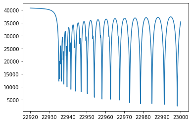
F0=rtrun(dtau,sourcef)

plt.plot(wav[::-1],F0)

We apply an instrumental response and planet/stellar rotation to the raw spectrum as

from exojax.spec import response
from exojax.utils.constants import c
import jax.numpy as jnp

wavd=jnp.linspace(22920,23000,500) #observational wavelength grid
nusd = 1.e8/wavd[::-1]

RV=10.0 #RV km/s
vsini=20.0 #Vsini km/s
u1=0.0 #limb darkening u1
u2=0.0 #limb darkening u2

R=100000.
beta=c/(2.0*np.sqrt(2.0*np.log(2.0))*R) #IP sigma need check

Frot=response.rigidrot(nus,F0,vsini,u1,u2)
F=response.ipgauss_sampling(nusd,nus,Frot,beta,RV)

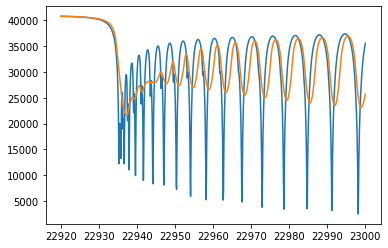
Finally, we get an emission spectrum model.

plt.plot(wav[::-1],F0)
plt.plot(wavd[::-1],F)

Save it!

np.savetxt("spectrum.txt",np.array([wavd,F]).T,delimiter=",")

This data is used in the next section “Reverse Modelling of an Emission Spectrum”.