Getting Started with Transmission Spectroscopy

Last update: March 15th (2025) Hajime Kawahara for v2.0

In this getting started guide, we will use ExoJAX to simulate a high-resolution transmission spectrum from an atmosphere with CO molecular absorption and hydrogen molecule CIA continuum absorption as the opacity sources. We will then add appropriate noise to the simulated spectrum to create a mock spectrum and perform spectral retrieval using NumPyro’s HMC NUTS.

First, we recommend 64-bit if you do not think about numerical errors. Use jax.config to set 64-bit. (But note that 32-bit is sufficient in most cases. Consider to use 32-bit (faster, less device memory) for your real use case.)

from jax import config
config.update("jax_enable_x64", True)

The following schematic figure explains how ExoJAX works; (1) loading databases (*db), (2) calculating opacity (opa), (3) running atmospheric radiative transfer (art), (4) applying operations on the spectrum (sop)

In this “getting started” guide, there are two opacity sources, CO and CIA. Their respective databases, mdb and cdb, are converted by opa into the opacity of each atmospheric layer, which is then used in the radiative transfer calculation performed by art. Finally, sop convolves instrumental profiles, generating the emission spectrum.

mdb/cdb –> opa –> art –> sop —> spectrum

This spectral model is incorporated into the probabilistic model in NumPyro, and retrieval is performed by sampling using HMC-NUTS.

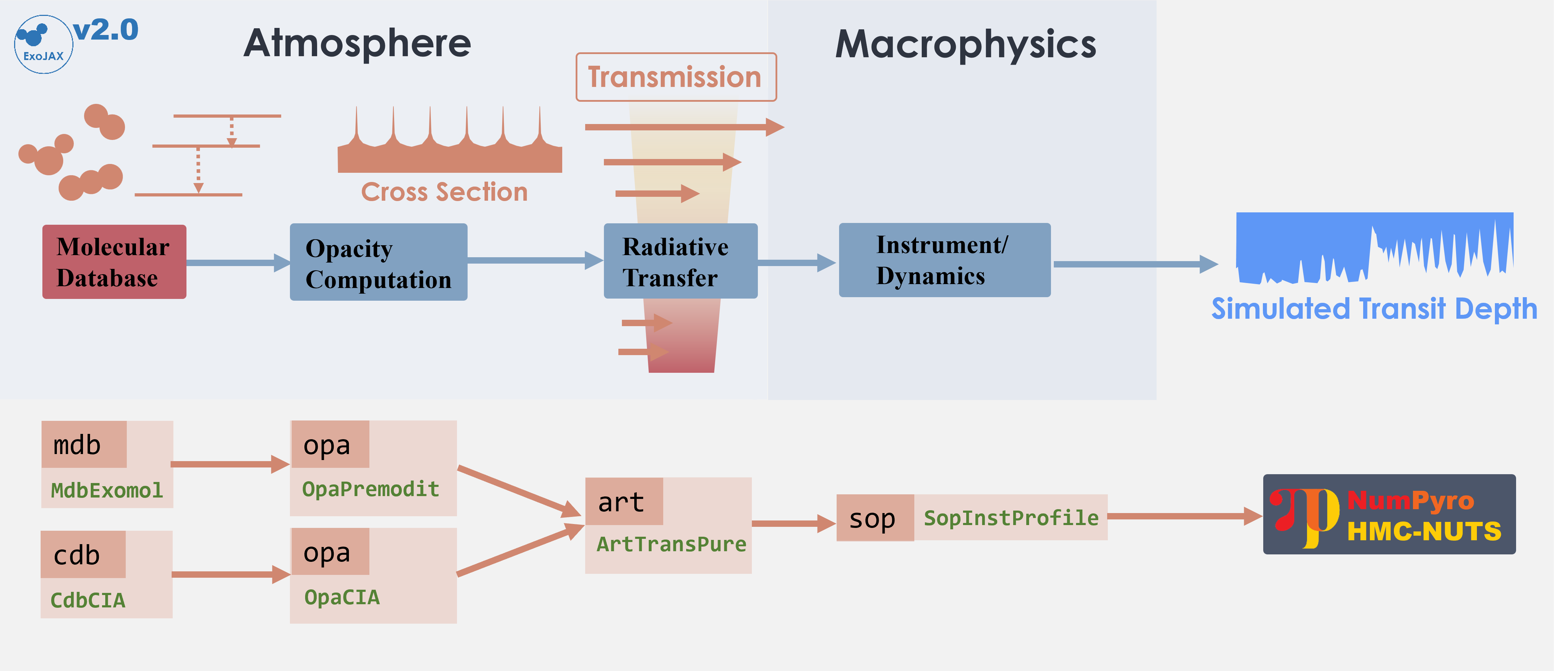
Figure. Structure of ExoJAX

1. Loading a molecular database using mdb

ExoJAX has an API for molecular databases, called mdb (or adb for atomic datbases). Prior to loading the database, define the wavenumber range first.

from exojax.utils.grids import wavenumber_grid

nu_grid, wav, resolution = wavenumber_grid(
    22920.0, 23000.0, 3500, unit="AA", xsmode="premodit"
)
print("Resolution=", resolution)

xsmode =  premodit
xsmode assumes ESLOG in wavenumber space: xsmode=premodit
Your wavelength grid is in *  descending  * order
The wavenumber grid is in ascending order by definition.
Please be careful when you use the wavelength grid.
Resolution= 1004211.9840291934

/home/kawahara/exojax/src/exojax/spec/unitconvert.py:82: UserWarning: Both input wavelength and output wavenumber are in ascending order.
  warnings.warn(

Then, let’s load the molecular database. We here use Carbon monoxide in Exomol. CO/12C-16O/Li2015 means Carbon monoxide/ isotopes = 12C + 16O / database name. You can check the database name in the ExoMol website (https://www.exomol.com/).

from exojax.spec.api import MdbExomol
mdb = MdbExomol(".database/CO/12C-16O/Li2015", nurange=nu_grid)

/home/kawahara/exojax/src/exojax/utils/molname.py:197: FutureWarning: e2s will be replaced to exact_molname_exomol_to_simple_molname.
  warnings.warn(
/home/kawahara/exojax/src/exojax/utils/molname.py:91: FutureWarning: exojax.utils.molname.exact_molname_exomol_to_simple_molname will be replaced to radis.api.exomolapi.exact_molname_exomol_to_simple_molname.
  warnings.warn(
/home/kawahara/exojax/src/exojax/utils/molname.py:91: FutureWarning: exojax.utils.molname.exact_molname_exomol_to_simple_molname will be replaced to radis.api.exomolapi.exact_molname_exomol_to_simple_molname.
  warnings.warn(

HITRAN exact name= (12C)(16O)
radis engine =  pytables
             => Downloading from http://www.exomol.com/db/CO/12C-16O/Li2015/12C-16O__Li2015.def
             => Downloading from http://www.exomol.com/db/CO/12C-16O/Li2015/12C-16O__Li2015.pf
             => Downloading from http://www.exomol.com/db/CO/12C-16O/Li2015/12C-16O__Li2015.states.bz2
             => Downloading from http://www.exomol.com/db/CO/12C-16O/12C-16O__H2.broad
             => Downloading from http://www.exomol.com/db/CO/12C-16O/12C-16O__He.broad
             => Downloading from http://www.exomol.com/db/CO/12C-16O/12C-16O__air.broad
             => Downloading from http://www.exomol.com/db/CO/12C-16O/12C-16O__self.broad
Error: Couldn't download .broad file at http://www.exomol.com/db/CO/12C-16O/12C-16O__self.broad and save.
             => Downloading from http://www.exomol.com/db/CO/12C-16O/12C-16O__Ar.broad
Error: Couldn't download .broad file at http://www.exomol.com/db/CO/12C-16O/12C-16O__Ar.broad and save.
             => Downloading from http://www.exomol.com/db/CO/12C-16O/12C-16O__CH4.broad
Error: Couldn't download .broad file at http://www.exomol.com/db/CO/12C-16O/12C-16O__CH4.broad and save.
             => Downloading from http://www.exomol.com/db/CO/12C-16O/12C-16O__CO.broad
Error: Couldn't download .broad file at http://www.exomol.com/db/CO/12C-16O/12C-16O__CO.broad and save.
             => Downloading from http://www.exomol.com/db/CO/12C-16O/12C-16O__CO2.broad
Error: Couldn't download .broad file at http://www.exomol.com/db/CO/12C-16O/12C-16O__CO2.broad and save.
             => Downloading from http://www.exomol.com/db/CO/12C-16O/12C-16O__H2.broad
             => Downloading from http://www.exomol.com/db/CO/12C-16O/12C-16O__H2O.broad
Error: Couldn't download .broad file at http://www.exomol.com/db/CO/12C-16O/12C-16O__H2O.broad and save.
             => Downloading from http://www.exomol.com/db/CO/12C-16O/12C-16O__N2.broad
Error: Couldn't download .broad file at http://www.exomol.com/db/CO/12C-16O/12C-16O__N2.broad and save.
             => Downloading from http://www.exomol.com/db/CO/12C-16O/12C-16O__NH3.broad
Error: Couldn't download .broad file at http://www.exomol.com/db/CO/12C-16O/12C-16O__NH3.broad and save.
             => Downloading from http://www.exomol.com/db/CO/12C-16O/12C-16O__NO.broad
Error: Couldn't download .broad file at http://www.exomol.com/db/CO/12C-16O/12C-16O__NO.broad and save.
             => Downloading from http://www.exomol.com/db/CO/12C-16O/12C-16O__O2.broad
Error: Couldn't download .broad file at http://www.exomol.com/db/CO/12C-16O/12C-16O__O2.broad and save.
             => Downloading from http://www.exomol.com/db/CO/12C-16O/12C-16O__NH3.broad
Error: Couldn't download .broad file at http://www.exomol.com/db/CO/12C-16O/12C-16O__NH3.broad and save.
             => Downloading from http://www.exomol.com/db/CO/12C-16O/12C-16O__CS.broad
Error: Couldn't download .broad file at http://www.exomol.com/db/CO/12C-16O/12C-16O__CS.broad and save.

Summary of broadening files downloaded:
    Success: ['H2' 'He' 'air' 'H2']
    Fail: ['self' 'Ar' 'CH4' 'CO' 'CO2' 'H2O' 'N2' 'NH3' 'NO' 'O2' 'NH3' 'CS']

Note: Caching states data to the pytables format. After the second time, it will become much faster.
Molecule:  CO
Isotopologue:  12C-16O
ExoMol database:  None
Local folder:  .database/CO/12C-16O/Li2015
Transition files:
     => File 12C-16O__Li2015.trans
             => Downloading from http://www.exomol.com/db/CO/12C-16O/Li2015/12C-16O__Li2015.trans.bz2
             => Caching the .trans.bz2 file to the pytables (.h5) format. After the second time, it will become much faster.
             => You can deleted the 'trans.bz2' file by hand.
Broadener:  H2
Broadening code level: a0

/home/kawahara/miniconda3/lib/python3.12/site-packages/radis-0.16-py3.12.egg/radis/api/exomolapi.py:687: AccuracyWarning: The default broadening parameter (alpha = 0.07 cm^-1 and n = 0.5) are used for J'' > 80 up to J'' = 152
  warnings.warn(

2. Computation of the Cross Section using opa

ExoJAX has various opacity calculator classes, so-called opa. Here, we use a memory-saved opa, OpaPremodit. We assume the robust tempreature range we will use is 500-1500K.

from exojax.spec.opacalc import OpaPremodit
opa = OpaPremodit(mdb, nu_grid, auto_trange=[500.0, 1500.0], dit_grid_resolution=1.0)

/home/kawahara/exojax/src/exojax/spec/opacalc.py:348: UserWarning: dit_grid_resolution is not None. Ignoring broadening_parameter_resolution.
  warnings.warn(

OpaPremodit: params automatically set.
default elower grid trange (degt) file version: 2
Robust range: 485.7803992045456 - 1514.171191195336 K
OpaPremodit: Tref_broadening is set to  866.0254037844389 K
# of reference width grid :  2
# of temperature exponent grid : 2
max value of  ngamma_ref_grid : 9.450919102366303
min value of  ngamma_ref_grid : 7.881095721823979
ngamma_ref_grid grid : [7.88109541 9.4509201 ]
max value of  n_Texp_grid : 0.658
min value of  n_Texp_grid : 0.5
n_Texp_grid grid : [0.49999997 0.65800005]

uniqidx: 0it [00:00, ?it/s]

Premodit: Twt= 1108.7151960064205 K Tref= 570.4914318566549 K
Making LSD:|####################| 100%
cross section (xsvector/xsmatrix) is calculated in the closed mode. The aliasing part cannnot be used.
wing cut width =  [15.12718787427093, 15.23298725175755] cm-1

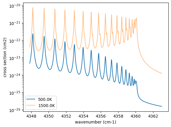
Then let’s compute cross section for two different temperature 500 and 1500 K for P=1.0 bar. opa.xsvector can do that!

P = 1.0  # bar
T_1 = 500.0  # K
xsv_1 = opa.xsvector(T_1, P)  # cm2

T_2 = 1500.0  # K
xsv_2 = opa.xsvector(T_2, P)  # cm2

Plot them. It can be seen that different lines are stronger at different temperatures.

import matplotlib.pyplot as plt

plt.plot(nu_grid, xsv_1, label=str(T_1) + "K")  # cm2
plt.plot(nu_grid, xsv_2, alpha=0.5, label=str(T_2) + "K")  # cm2
plt.yscale("log")
plt.legend()
plt.xlabel("wavenumber (cm-1)")
plt.ylabel("cross section (cm2)")
plt.show()

3. Atmospheric Radiative Transfer

ExoJAX can solve the radiative transfer and derive the transmission spectrum. To do so, ExoJAX has art class. ArtTransPure means Atomospheric Radiative Transfer for Transmission with Pure absorption. So, ArtTransPure does not include scattering. You can choose either the trapezoid or Simpson’s rule as the integration scheme. The default setting is integration="simpson". We set the number of the atmospheric layer to 200 (nlayer) and the pressure at bottom and top atmosphere to 1 and 1.e-11 bar.

from exojax.spec.atmrt import ArtTransPure

art = ArtTransPure(
    pressure_btm=1.0e1,
    pressure_top=1.0e-11,
    nlayer=200,
)

integration:  simpson
Simpson integration, uses the chord optical depth at the lower boundary and midppoint of the layers.

/home/kawahara/exojax/src/exojax/spec/dtau_mmwl.py:13: FutureWarning: dtau_mmwl might be removed in future.
  warnings.warn("dtau_mmwl might be removed in future.", FutureWarning)
/home/kawahara/exojax/src/exojax/spec/atmrt.py:53: UserWarning: nu_grid is not given. specify nu_grid when using 'run'
  warnings.warn(

Let’s assume the power law temperature model, within 500 - 1500 K.

\(T = T_0 P^\alpha\)

where \(T_0=1200\) K and \(\alpha=0.1\).

art.change_temperature_range(500.0, 1500.0)
Tarr = art.powerlaw_temperature(1200.0, 0.1)

Also, the mass mixing ratio of CO (MMR) should be defined.

mmr_profile = art.constant_mmr_profile(0.01)

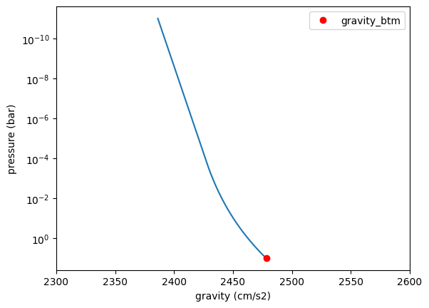
Surface gravity is also important quantity of the atmospheric model, which is a function of planetary radius and mass. Unlike in the case of the emission spectrum, the transmission spectrum is affected by the opacity from the lower to the upper layers of the atmosphere. Therefore, it is better to calculate gravity as a function of altitude. To achieve this, the gravity and radius at the bottom of the atmospheric layer are specified as gravity_btm and radius_btm, respectively, and the layer-by-layer gravity profile is computed using art.gravity_profile.

import jax.numpy as jnp
from exojax.utils.astrofunc import gravity_jupiter
from exojax.utils.constants import RJ
gravity_btm = gravity_jupiter(1.0, 1.0)
radius_btm = RJ

mmw = 2.33*jnp.ones_like(art.pressure)  # mean molecular weight of the atmosphere
gravity = art.gravity_profile(Tarr, mmw, radius_btm, gravity_btm)

When visualized, it looks like this.

plt.plot(gravity, art.pressure)
plt.plot(gravity_btm, art.pressure[-1], "ro", label="gravity_btm")
plt.yscale("log")
plt.xlim(2300,2600)
plt.gca().invert_yaxis()
plt.xlabel("gravity (cm/s2)")
plt.ylabel("pressure (bar)")
plt.legend()
plt.show()

In addition to the CO cross section, we would consider collisional induced absorption (CIA) as a continuum opacity. cdb class can be used.

from exojax.spec.contdb import CdbCIA
from exojax.spec.opacont import OpaCIA

cdb = CdbCIA(".database/H2-H2_2011.cia", nurange=nu_grid)
opacia = OpaCIA(cdb, nu_grid=nu_grid)

H2-H2

Before running the radiative transfer, we need cross sections for layers, called xsmatrix for CO and logacia_matrix for CIA (strictly speaking, the latter is not cross section but coefficient because CIA intensity is proportional density square). See here for the details.

xsmatrix = opa.xsmatrix(Tarr, art.pressure)
logacia_matrix = opacia.logacia_matrix(Tarr)

Convert them to opacity

dtau_CO = art.opacity_profile_xs(xsmatrix, mmr_profile, mdb.molmass, gravity)
vmrH2 = 0.855  # VMR of H2
dtaucia = art.opacity_profile_cia(logacia_matrix, Tarr, vmrH2, vmrH2, mmw[:, None], gravity)

Add two opacities.

dtau = dtau_CO + dtaucia

gravity_btm

2478.57730044555

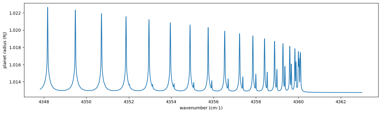
Then, run the radiative transfer. As you can see, the emission spectrum has been generated. This spectrum shows a region near 4360 cm-1, or around 22940 AA, where CO features become increasingly dense. This region is referred to as the band head. If you’re interested in why the band head occurs, please refer to Quatum states of Carbon Monoxide and Fortrat Diagram.

Rp2 = art.run(dtau, Tarr, mmw, radius_btm, gravity_btm)
Rp = jnp.sqrt(Rp2)

fig = plt.figure(figsize=(15, 4))
plt.plot(nu_grid, Rp)
plt.xlabel("wavenumber (cm-1)")
plt.ylabel("planet radius (RJ)")
plt.show()

To examine the contribution of each atmospheric layer to the transmission spectrum, one can, for example, look at the optical depth along the chord direction. This can be done as follows:

from exojax.spec.opachord import chord_geometric_matrix
from exojax.spec.opachord import chord_optical_depth

normalized_height, normalized_radius_lower = art.atmosphere_height(Tarr, mmw, radius_btm, gravity_btm)
cgm = chord_geometric_matrix(normalized_height, normalized_radius_lower)
dtau_chord = chord_optical_depth(cgm, dtau)

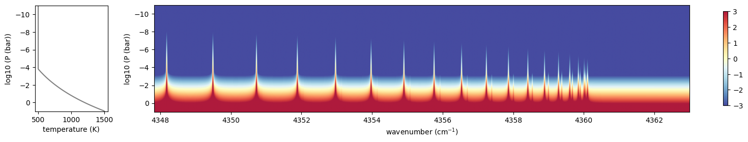
By plotting the data, it becomes clear that in the case of transmitted light, information from a wide range of atmospheric layers, from the upper to the lower layers, is included.

from exojax.plot.atmplot import plottau
plottau(nu_grid, dtau_chord, Tarr, art.pressure)

/home/kawahara/exojax/src/exojax/plot/atmplot.py:51: SyntaxWarning: invalid escape sequence 'm'
  plt.xlabel("wavenumber ($mathrm{cm}^{-1}$)")
/home/kawahara/exojax/src/exojax/plot/atmplot.py:68: SyntaxWarning: invalid escape sequence 'm'
  labelx["um"] = "wavelength ($mu mathrm{m}$)"
/home/kawahara/exojax/src/exojax/plot/atmplot.py:70: SyntaxWarning: invalid escape sequence 'A'
  labelx["AA"] = "wavelength ($AA$)"
/home/kawahara/exojax/src/exojax/plot/atmplot.py:71: SyntaxWarning: invalid escape sequence 'm'
  labelx["cm-1"] = "wavenumber ($mathrm{cm}^{-1}$)"
/home/kawahara/exojax/src/exojax/plot/atmplot.py:24: UserWarning: nugrid looks in log scale, results in a wrong X-axis value. Use log10(nugrid) instead.
  warnings.warn(

4. Spectral Operators:　instrumental profile, Doppler velocity shift and so on, any operation on spectra.

The above spectrum is called “raw spectrum” in ExoJAX. The effects applied to the raw spectrum is handled in ExoJAX by the spectral operator (sop).

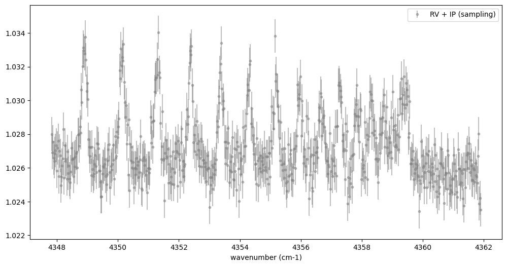
Then, the instrumental profile with relative radial velocity shift is applied. Also, we need to match the computed spectrum to the data grid. This process is called sampling (but just interpolation though). Below, let’s perform a simulation that includes noise for use in later analysis.

from exojax.spec.specop import SopInstProfile
from exojax.utils.instfunc import resolution_to_gaussian_std

sop_inst = SopInstProfile(nu_grid, vrmax=1000.0)

RV = 40.0  # km/s
resolution_inst = 30000.0
beta_inst = resolution_to_gaussian_std(resolution_inst)
Rp2_inst = sop_inst.ipgauss(Rp2, beta_inst)
nu_obs = nu_grid[::5][:-50]


from numpy.random import normal
noise = 0.001
Fobs = sop_inst.sampling(Rp2_inst, RV, nu_obs) + normal(0.0, noise, len(nu_obs))

fig = plt.figure(figsize=(12, 6))
ax = fig.add_subplot(111)

plt.errorbar(nu_obs, Fobs, noise, fmt=".", label="RV + IP (sampling)", color="gray",alpha=0.5)
plt.xlabel("wavenumber (cm-1)")
plt.legend()
plt.show()

5. Retrieval of a Transmission Spectrum

Next, let’s perform a “retrieval” on the simulated spectrum created above. Retrieval involves estimating the parameters of an atmospheric model in the form of a posterior distribution based on the spectrum. To do this, we first need a model. Here, we have compiled the forward modeling steps so far and defined the model as follows. The spectral model has six parameters.

def fspec(T0, alpha, mmr, radius_btm, gravity_btm, RV):
    """ computes planet radius sqaure spectrum

    Args:
        T0 (float): temperature at 1 bar
        alpha (float): power law index of temperature
        mmr (float): Mass mixing ratio of CO
        radius_btm (float): radius at the bottom in cm
        gravity_btm (float): gravity at the bottom in cm/s2
        RV (float): radial velocity in km/s

    Returns:
        _type_: _description_
    """

    Tarr = art.powerlaw_temperature(T0, alpha)
    gravity = art.gravity_profile(Tarr, mmw, radius_btm, gravity_btm)

    #molecule
    xsmatrix = opa.xsmatrix(Tarr, art.pressure)
    mmr_arr = art.constant_mmr_profile(mmr)
    dtau = art.opacity_profile_xs(xsmatrix, mmr_arr, opa.mdb.molmass, gravity)
    #continuum
    logacia_matrix = opacia.logacia_matrix(Tarr)
    dtaucH2H2 = art.opacity_profile_cia(logacia_matrix, Tarr, vmrH2, vmrH2,
                                        mmw[:, None], gravity)
    #total tau
    dtau = dtau + dtaucH2H2
    Rp2 = art.run(dtau, Tarr, mmw, radius_btm, gravity_btm)
    Rp2_inst = sop_inst.ipgauss(Rp2, beta_inst)

    mu = sop_inst.sampling(Rp2_inst, RV, nu_obs)
    return mu

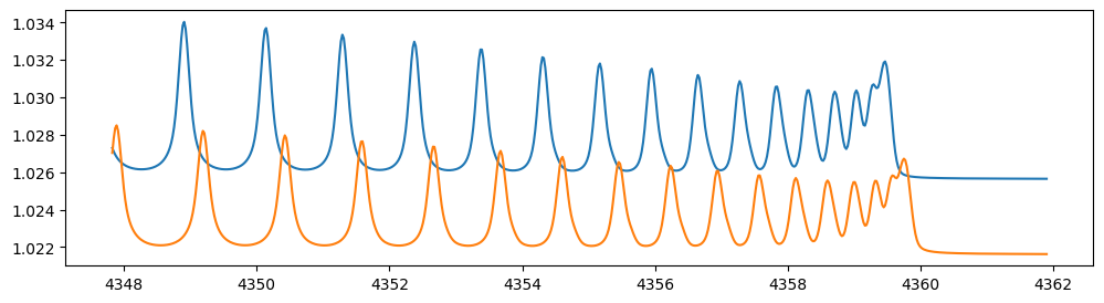
Let’s verify that spectra are being generated from fspec with various parameter sets.

fig = plt.figure(figsize=(12, 3))

plt.plot(nu_obs, fspec(1200.0, 0.09, 0.01, RJ, gravity_jupiter(1.0, 1.0), 40.0),label="model")
plt.plot(nu_obs, fspec(1400.0, 0.12, 0.01, RJ, gravity_jupiter(1.0, 1.3), 20.0),label="model")

[<matplotlib.lines.Line2D at 0x745a21794980>]

NumPyro is a probabilistic programming language (PPL), which requires the definition of a probabilistic model. In the probabilistic model model_prob defined below, the prior distributions of each parameter are specified. The previously defined spectral model is used within this probabilistic model as a function that provides the mean \(\mu\). The spectrum is assumed to be generated according to a Gaussian distribution with this mean and a standard deviation \(\sigma\). i.e. \(f(\nu_i) \sim \mathcal{N}(\mu(\nu_i; {\bf p}), \sigma^2 I)\), where \({\bf p}\) is the spectral model parameter set, which are the arguments of fspec.

from numpyro.infer import MCMC, NUTS
import numpyro.distributions as dist
import numpyro
from jax import random

/home/kawahara/miniconda3/lib/python3.12/site-packages/tqdm/auto.py:21: TqdmWarning: IProgress not found. Please update jupyter and ipywidgets. See https://ipywidgets.readthedocs.io/en/stable/user_install.html
  from .autonotebook import tqdm as notebook_tqdm

def model_prob(spectrum):

    #atmospheric/spectral model parameters priors
    logg = numpyro.sample('logg', dist.Uniform(3.0, 4.0))
    RV = numpyro.sample('RV', dist.Uniform(35.0, 45.0))
    mmr = numpyro.sample('MMR', dist.Uniform(0.0, 0.015))
    T0 = numpyro.sample('T0', dist.Uniform(1000.0, 1500.0))
    alpha = numpyro.sample('alpha', dist.Uniform(0.05, 0.2))
    radius_btm = numpyro.sample('rb', dist.Normal(1.0,0.05))

    mu = fspec(T0, alpha, mmr, radius_btm*RJ, 10**logg, RV)

    #noise model parameters priors
    sigmain = numpyro.sample('sigmain', dist.Exponential(1000.0))

    numpyro.sample('spectrum', dist.Normal(mu, sigmain), obs=spectrum)

Now, let’s define NUTS and start sampling.

rng_key = random.PRNGKey(0)
rng_key, rng_key_ = random.split(rng_key)
num_warmup, num_samples = 500, 1000
#kernel = NUTS(model_prob, forward_mode_differentiation=True)
kernel = NUTS(model_prob, forward_mode_differentiation=False)

Since this process will take several hours, feel free to go for a long lunch break!

mcmc = MCMC(kernel, num_warmup=num_warmup, num_samples=num_samples)
mcmc.run(rng_key_, spectrum=Fobs)
mcmc.print_summary()

sample: 100%|██████████| 1500/1500 [2:23:08<00:00,  5.73s/it, 127 steps of size 1.14e-02. acc. prob=0.94]

                mean       std    median      5.0%     95.0%     n_eff     r_hat
       MMR      0.01      0.00      0.01      0.01      0.01    309.22      1.00
        RV     39.79      0.16     39.79     39.53     40.05    709.96      1.00
        T0   1130.71     53.36   1126.14   1044.55   1215.44    396.74      1.00
     alpha      0.09      0.01      0.09      0.08      0.11    309.49      1.00
      logg      3.37      0.03      3.37      3.32      3.42    402.09      1.00
        rb      1.00      0.05      1.00      0.91      1.09    670.37      1.00
   sigmain      0.00      0.00      0.00      0.00      0.00    760.18      1.00

Number of divergences: 0

After returning from your long lunch, if you’re lucky and the sampling is complete, let’s write a predictive model for the spectrum.

from numpyro.diagnostics import hpdi
from numpyro.infer import Predictive
import jax.numpy as jnp

# SAMPLING
posterior_sample = mcmc.get_samples()
pred = Predictive(model_prob, posterior_sample, return_sites=['spectrum'])
predictions = pred(rng_key_, spectrum=None)
median_mu1 = jnp.median(predictions['spectrum'], axis=0)
hpdi_mu1 = hpdi(predictions['spectrum'], 0.9)

fig, ax = plt.subplots(nrows=1, ncols=1, figsize=(15, 4.5))
ax.plot(nu_obs, median_mu1, color='C1')
ax.fill_between(nu_obs,
                hpdi_mu1[0],
                hpdi_mu1[1],
                alpha=0.3,
                interpolate=True,
                color='C1',
                label='90% area')
ax.errorbar(nu_obs, Fobs, noise, fmt=".", label="mock spectrum", color="black",alpha=0.5)
plt.xlabel('wavenumber (cm-1)', fontsize=16)
plt.legend(fontsize=14)
plt.tick_params(labelsize=14)
plt.show()

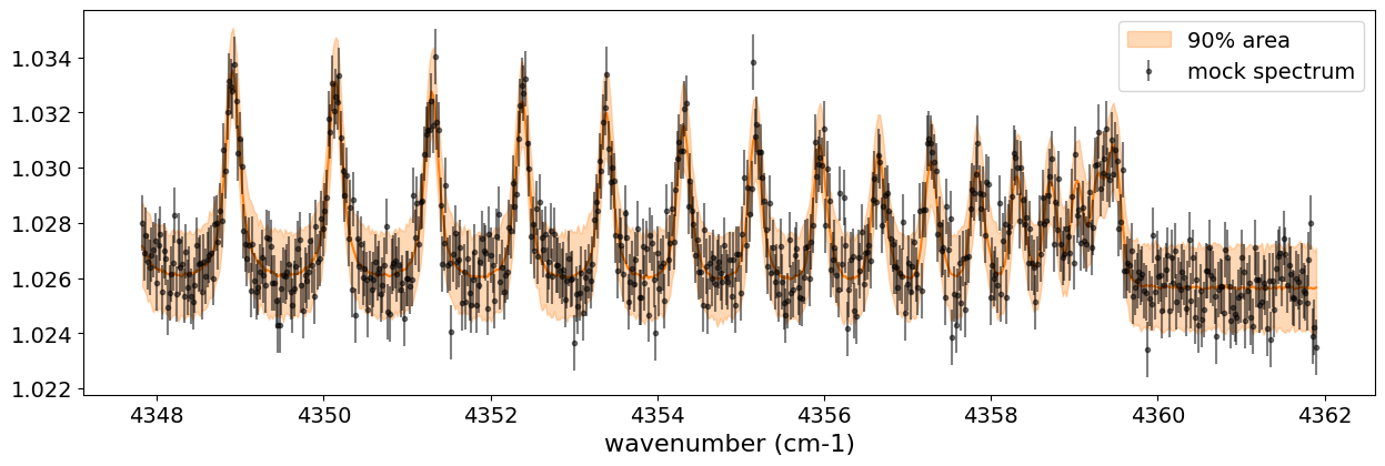
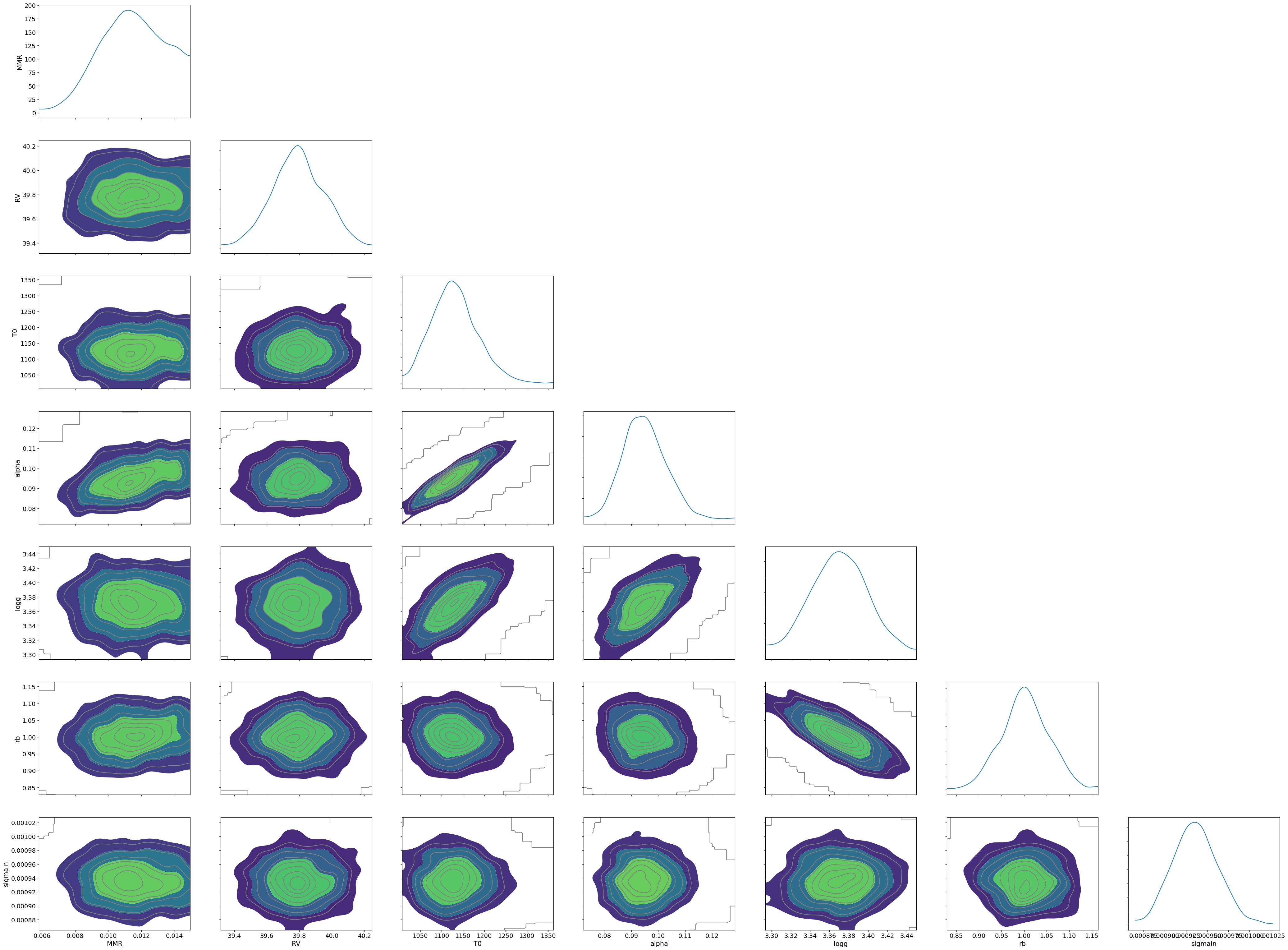
You can see that the predictions are working very well! Let’s also display a corner plot. Here, we’ve used ArviZ for visualization.

import arviz
pararr = ['T0', 'alpha', 'logg', 'MMR', 'radius_btm', 'RV']
arviz.plot_pair(arviz.from_numpyro(mcmc),
                kind='kde',
                divergences=False,
                marginals=True)
plt.show()

Further Information

Correlated noise can be introduced using a Gaussian process, and parameter estimation can be performed using SVI or Nested Sampling, just as in the case of emission spectra. See below for details.

• Including GP in an emission spectrum

• SVI for an emission spectrum

• Neste Sampling for an emission spectrum

Not enough GPU device memory? In that case, you can perform wavenumber splitting. See below for details.

• wavenumber stitching

Want to analyze JWST data? The Gallery and the following repositories may be helpful.

• ExoJAX gallery

• exojaxample_WASP39b by Shotaro Tada (@sh-tada)

That’s it.