Transmission Spectroscopy
In transmission spectroscopy, the spectrum of the transit depth is measured. The transit depth is the square of the ratio between the planet’s radius
and the star’s radius. Accordingly, ExoJAX calculates the square of the planet’s radius.
\(R_{p,\nu}^2 = R_{0}^2 + \Delta R_{p,\nu}^2\),
where \(R_0=\underline{r}_{N-1}\) is the lower boundary of the bottom layer. Atmosphere below this point must remain completely opaque. The contribution of the atmospheric layers to the transit radius squared is expressed as
\(\Delta R_{p,\nu}^2 \equiv 2 \int_{R_{0}}^\infty [ 1 - \mathcal{T}_\nu(r)] r d r \approx 2 \int_{\underline{r}_{N-1}}^{\overline{r}_0} [ 1 - \mathcal{T}_\nu(r)] r d r\),
where \(\mathcal{T}_\nu(r) = e^{-t(r)}\) is the transmission at r and \(t(r)\) is the chord optical depth at r and \(\underline{r}_0\) is the lower boundary of the top of atmosphere.
Uses ArtTransPure class
To calculate the transmission spectrum in ExoJAX, the ArtTransPure class is convenient.
For chord integration, one can choose either Simpson’s method or the trapezoidal method from the integration options.
Here is the example of the computation of the transmission radius. We here use Simpson’s rule for the chord integration.
In transmission spectroscopy, assuming a constant gravity across the layers is often not a good approximation.
The gravity_profile instance in the ArtTransPure class allows for easy calculation of the gravity profile, addressing this concern in ExoJAX.
from exojax.rt import ArtTransPure
from exojax.utils.constants import RJ

art = ArtTransPure(pressure_top=1.e-8, pressure_btm=1.e2, nlayer=100, integration="simpson") # integration="trapezoid" if you want
art.change_temperature_range(400.0, 1500.0)
Tarr = art.powerlaw_temperature(1300.0, 0.1)
mmr_arr = art.constant_mmr_profile(0.1) # constant mass mixing ratio profile
mmw = 2.33 * np.ones_like(art.pressure) # mean molecular weight profile
gravity_btm = 2478.57
radius_btm = RJ
gravity = art.gravity_profile(Tarr, mmw, radius_btm, gravity_btm) # computes gravity profile

opa = OpaPremodit(mdb=mdb,
                  nu_grid=nu_grid,
                  auto_trange=[art.Tlow, art.Thigh])

xsmatrix = opa.xsmatrix(Tarr, art.pressure)

dtau = art.opacity_profile_xs(xsmatrix, mmr_arr, opa.mdb.molmass,gravity)
Rp2 = art.run(dtau, Tarr, mmw, radius_btm, gravity_btm)
🎃 See Getting Started with simulating the Transmission Spectrum as a tutorial.
Real Example
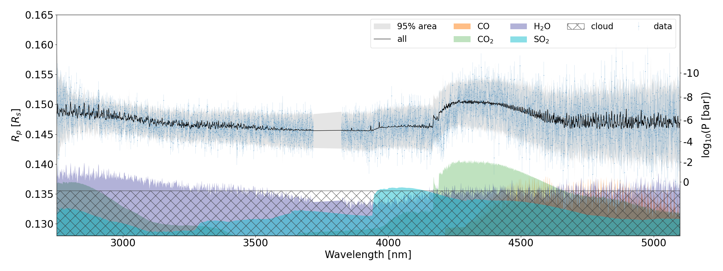
Figure. Real HMC-NUTS analysis of the transmission spectrum of WASP-39b observed by JWST/NIRSpec G395H (Paper II ).
An example of calculating the actual transmission spectrum of the hot Saturn WASP-39b observed by JWST can be found in the following repository:
exojaxample_WASP39b By Shotaro Tada, as used in Paper II