Stochastic Variation Inference with Auto Guide Generation of an Emission Spectrum Using NumPyro
Last update: September 25th (2025) Hajime Kawahara for v2.2.0
In this guide, we perform retrieval of an emission spectrum using stochastic variational inference (SVI) with automatic guide generation. The structure is the same as in the getting started guide, except that we use SVI instead of HMC-NUTS; i.e. we will use ExoJAX to simulate a high-resolution emission spectrum from an atmosphere with CO molecular absorption and hydrogen molecule CIA continuum absorption as the opacity sources. We will then add appropriate noise to the simulated spectrum to create a mock spectrum and perform spectral retrieval using the nested sampling.
Here, we use SVI and …, which is bundled with NumPyro, as the sampler. Notably, apart from the final retrieval step, most of the code remains the same as in the HMC-NUTS case.
First, we recommend 64-bit if you do not think about numerical errors. Use jax.config to set 64-bit. (But note that 32-bit is sufficient in most cases. Consider to use 32-bit (faster, less device memory) for your real use case.)
from jax import config
config.update("jax_enable_x64", True)
The following schematic figure explains how ExoJAX works; (1) loading
databases (*db), (2) calculating opacity (opa), (3) running
atmospheric radiative transfer (art), (4) applying operations on the
spectrum (sop)
In this guide, there are two opacity sources, CO and CIA. Their
respective databases, mdb and cdb, are converted by opa into
the opacity of each atmospheric layer, which is then used in the
radiative transfer calculation performed by art. Finally, sop
convolves the rotational effects and instrumental profiles, generating
the emission spectrum.
mdb/cdb –> opa –> art –> sop —> spectrum
This spectral model is incorporated into the probabilistic model in NumPyro with JAXNS, and retrieval is performed by sampling using nested sampling.
1. Loading a molecular database using mdb
ExoJAX has an API for molecular databases, called mdb (or adb
for atomic datbases). Prior to loading the database, define the
wavenumber range first.
from exojax.utils.grids import wavenumber_grid

nu_grid, wav, resolution = wavenumber_grid(
    22920.0, 23000.0, 3500, unit="AA", xsmode="premodit"
)
print("Resolution=", resolution)
xsmode =  premodit
xsmode assumes ESLOG in wavenumber space: xsmode=premodit
Your wavelength grid is in *  descending  * order
The wavenumber grid is in ascending order by definition.
Please be careful when you use the wavelength grid.
Resolution= 1004211.9840291934
/home/kawahara/exojax/src/exojax/utils/grids.py:85: UserWarning: Both input wavelength and output wavenumber are in ascending order.
  warnings.warn(
Then, let’s load the molecular database. We here use Carbon monoxide in
Exomol. CO/12C-16O/Li2015 means
Carbon monoxide/ isotopes = 12C + 16O / database name. You can check
the database name in the ExoMol website (https://www.exomol.com/).
from exojax.database.exomol.api import MdbExomol
mdb = MdbExomol(".database/CO/12C-16O/Li2015", nurange=nu_grid)
molmass = mdb.molmass
HITRAN exact name= (12C)(16O)
radis engine =  vaex
Molecule:  CO
Isotopologue:  12C-16O
ExoMol database:  None
Local folder:  .database/CO/12C-16O/Li2015
Transition files:
     => File 12C-16O__Li2015.trans
Broadener:  H2
Broadening code level: a0
/home/kawahara/exojax/src/exojax/utils/molname.py:197: FutureWarning: e2s will be replaced to exact_molname_exomol_to_simple_molname.
  warnings.warn(
/home/kawahara/exojax/src/exojax/utils/molname.py:91: FutureWarning: exojax.utils.molname.exact_molname_exomol_to_simple_molname will be replaced to radis.api.exomolapi.exact_molname_exomol_to_simple_molname.
  warnings.warn(
/home/kawahara/exojax/src/exojax/utils/molname.py:91: FutureWarning: exojax.utils.molname.exact_molname_exomol_to_simple_molname will be replaced to radis.api.exomolapi.exact_molname_exomol_to_simple_molname.
  warnings.warn(
/home/kawahara/anaconda3/lib/python3.10/site-packages/radis/api/exomolapi.py:727: AccuracyWarning: The default broadening parameter (alpha = 0.07 cm^-1 and n = 0.5) are used for J'' > 80 up to J'' = 152
  warnings.warn(
2. Computation of the Cross Section using opa
ExoJAX has various opacity calculator classes, so-called opa. Here,
we use a memory-saved opa, OpaPremodit. We assume the robust
tempreature range we will use is 500-1500K.
from exojax.opacity import OpaPremodit
snap = mdb.to_snapshot()
del mdb
opa = OpaPremodit.from_snapshot(snap, nu_grid, auto_trange=[500.0, 1500.0], dit_grid_resolution=1.0)
/home/kawahara/exojax/src/exojax/opacity/premodit/core.py:28: UserWarning: dit_grid_resolution is not None. Ignoring broadening_parameter_resolution.
  warnings.warn(
default elower grid trange (degt) file version: 2
Robust range: 485.7803992045456 - 1514.171191195336 K
max value of  ngamma_ref_grid : 9.450919102366303
min value of  ngamma_ref_grid : 7.881095721823979
ngamma_ref_grid grid : [7.88109541 9.4509201 ]
max value of  n_Texp_grid : 0.658
min value of  n_Texp_grid : 0.5
n_Texp_grid grid : [0.49999997 0.65800005]
uniqidx: 0it [00:00, ?it/s]
Premodit: Twt= 1108.7151960064205 K Tref= 570.4914318566549 K
Making LSD:|####################| 100%
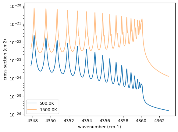
Then let’s compute cross section for two different temperature 500 and 1500 K for P=1.0 bar. opa.xsvector can do that!
P = 1.0  # bar
T_1 = 500.0  # K
xsv_1 = opa.xsvector(T_1, P)  # cm2

T_2 = 1500.0  # K
xsv_2 = opa.xsvector(T_2, P)  # cm2
Plot them. It can be seen that different lines are stronger at different temperatures.
import matplotlib.pyplot as plt

plt.plot(nu_grid, xsv_1, label=str(T_1) + "K")  # cm2
plt.plot(nu_grid, xsv_2, alpha=0.5, label=str(T_2) + "K")  # cm2
plt.yscale("log")
plt.legend()
plt.xlabel("wavenumber (cm-1)")
plt.ylabel("cross section (cm2)")
plt.show()
3. Atmospheric Radiative Transfer
ExoJAX can solve the radiative transfer and derive the emission
spectrum. To do so, ExoJAX has art class. ArtEmisPure means
Atomospheric Radiative Transfer for Emission with Pure absorption. So,
ArtEmisPure does not include scattering. We set the number of the
atmospheric layer to 200 (nlayer) and the pressure at bottom and top
atmosphere to 100 and 1.e-5 bar.
Since v1.5, one can choose the rtsolver (radiative transfer solver) from
the flux-based 2 stream solver (fbase2st) and the intensity-based
n-stream sovler (ibased). Use rtsolver option. In the latter
case, the number of the stream (nstream) can be specified. Note that
the default rtsolver for the pure absorption (i.e. no scattering nor
reflection) has been ibased since v1.5. In our experience,
ibased is faster and more accurate than fbased.
from exojax.rt import ArtEmisPure

art = ArtEmisPure(
    nu_grid=nu_grid,
    pressure_btm=1.0e1,
    pressure_top=1.0e-5,
    nlayer=100,
    rtsolver="ibased",
    nstream=8,
)
rtsolver:  ibased
Intensity-based n-stream solver, isothermal layer (e.g. NEMESIS, pRT like)
Let’s assume the power law temperature model, within 500 - 1500 K.
\(T = T_0 P^\alpha\)
where \(T_0=1200\) K and \(\alpha=0.1\).
art.change_temperature_range(500.0, 1500.0)
Tarr = art.powerlaw_temperature(1200.0, 0.1)
Also, the mass mixing ratio of CO (MMR) should be defined.
mmr_profile = art.constant_mmr_profile(0.01)
Surface gravity is also important quantity of the atmospheric model, which is a function of planetary radius and mass. Here we assume 1 RJ and 10 MJ.
from exojax.utils.astrofunc import gravity_jupiter

gravity = gravity_jupiter(1.0, 10.0)
In addition to the CO cross section, we would consider collisional
induced
absorption
(CIA) as a continuum opacity. cdb class can be used.
from exojax.database.contdb  import CdbCIA
from exojax.opacity import OpaCIA

cdb = CdbCIA(".database/H2-H2_2011.cia", nurange=nu_grid)
opacia = OpaCIA(cdb, nu_grid=nu_grid)
H2-H2
Before running the radiative transfer, we need cross sections for
layers, called xsmatrix for CO and logacia_matrix for CIA
(strictly speaking, the latter is not cross section but coefficient
because CIA intensity is proportional density square). See
here for the details.
xsmatrix = opa.xsmatrix(Tarr, art.pressure)
logacia_matrix = opacia.logacia_matrix(Tarr)
Convert them to opacity
dtau_CO = art.opacity_profile_xs(xsmatrix, mmr_profile, molmass, gravity)
vmrH2 = 0.855  # VMR of H2
mmw = 2.33  # mean molecular weight of the atmosphere
dtaucia = art.opacity_profile_cia(logacia_matrix, Tarr, vmrH2, vmrH2, mmw, gravity)
Add two opacities.
dtau = dtau_CO + dtaucia
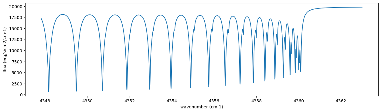
Then, run the radiative transfer. As you can see, the emission spectrum has been generated. This spectrum shows a region near 4360 cm-1, or around 22940 AA, where CO features become increasingly dense. This region is referred to as the band head. If you’re interested in why the band head occurs, please refer to Quatum states of Carbon Monoxide and Fortrat Diagram.
F = art.run(dtau, Tarr)

fig = plt.figure(figsize=(15, 4))
plt.plot(nu_grid, F)
plt.xlabel("wavenumber (cm-1)")
plt.ylabel("flux (erg/s/cm2/cm-1)")
plt.show()
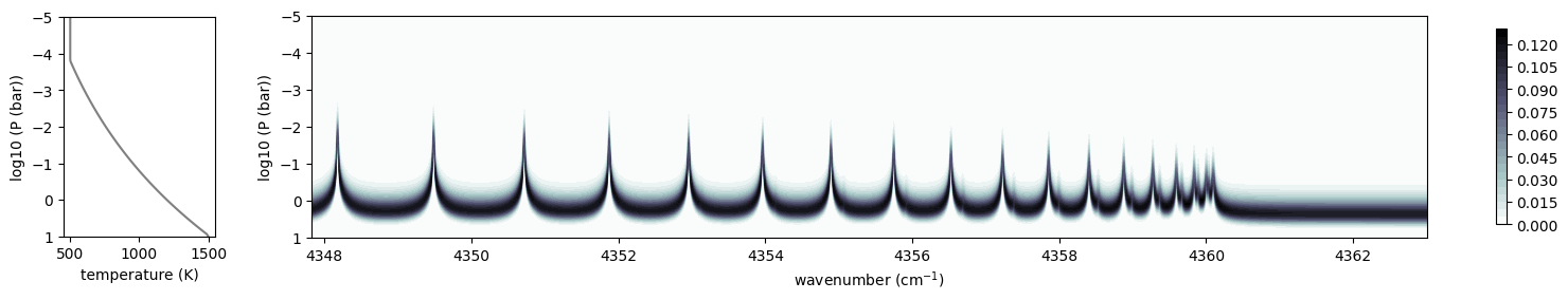
You can check the contribution function too! You should check if the
dominant contribution is within the layer. If not, you need to change
pressure_top and pressure_btm in ArtEmisPure
from exojax.plot.atmplot import plotcf
cf = plotcf(nu_grid, dtau, Tarr, art.pressure, art.dParr)
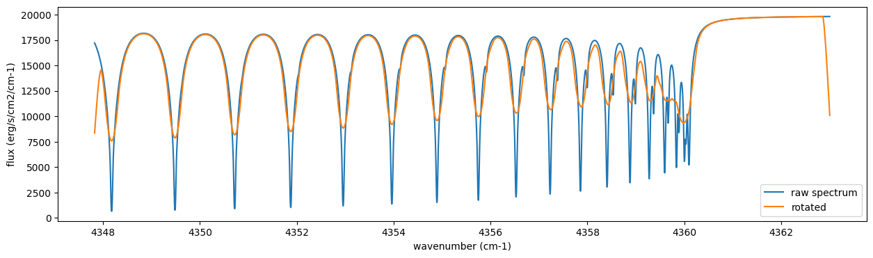
4. Spectral Operators: rotational broadening, instrumental profile, Doppler velocity shift and so on, any operation on spectra.
The above spectrum is called “raw spectrum” in ExoJAX. The effects
applied to the raw spectrum is handled in ExoJAX by the spectral
operator (sop). First, we apply the spin rotational broadening of a
planet.
from exojax.postproc.specop import SopRotation

sop_rot = SopRotation(nu_grid, vsini_max=100.0)

vsini = 10.0
u1 = 0.0
u2 = 0.0
Frot = sop_rot.rigid_rotation(F, vsini, u1, u2)
fig = plt.figure(figsize=(15, 4))
plt.plot(nu_grid, F, label="raw spectrum")
plt.plot(nu_grid, Frot, label="rotated")
plt.xlabel("wavenumber (cm-1)")
plt.ylabel("flux (erg/s/cm2/cm-1)")
plt.legend()
plt.show()
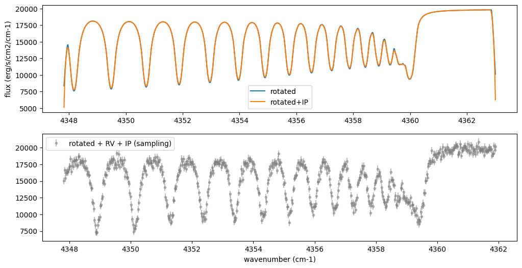
Then, the instrumental profile with relative radial velocity shift is
applied. Also, we need to match the computed spectrum to the data grid.
This process is called sampling (but just interpolation though).
Below, let’s perform a simulation that includes noise for use in later
analysis.
from exojax.postproc.specop import SopInstProfile
from exojax.utils.instfunc import resolution_to_gaussian_std

sop_inst = SopInstProfile(nu_grid, vrmax=1000.0)

RV = 40.0  # km/s
resolution_inst =70000.0
beta_inst = resolution_to_gaussian_std(resolution_inst)
Finst = sop_inst.ipgauss(Frot, beta_inst)
nu_obs = nu_grid[::5][:-50]


from numpy.random import normal
noise = 500.0
Fobs = sop_inst.sampling(Finst, RV, nu_obs) + normal(0.0, noise, len(nu_obs))
fig = plt.figure(figsize=(12, 6))
ax = fig.add_subplot(211)
plt.plot(nu_grid, Frot, label="rotated")
plt.plot(nu_grid, Finst, label="rotated+IP")
plt.ylabel("flux (erg/s/cm2/cm-1)")
plt.legend()
ax = fig.add_subplot(212)
plt.errorbar(nu_obs, Fobs, noise, fmt=".", label="rotated + RV + IP (sampling)", color="gray",alpha=0.5)
plt.xlabel("wavenumber (cm-1)")
plt.legend()
plt.show()
5. Retrieval of an Emission Spectrum
Next, let’s perform a “retrieval” on the simulated spectrum created above. Retrieval involves estimating the parameters of an atmospheric model in the form of a posterior distribution based on the spectrum. To do this, we first need a model. Here, we have compiled the forward modeling steps so far and defined the model as follows. The spectral model has six parameters.
def fspec(T0, alpha, mmr, g, RV, vsini):
    #molecule
    Tarr = art.powerlaw_temperature(T0, alpha)
    xsmatrix = opa.xsmatrix(Tarr, art.pressure)
    mmr_arr = art.constant_mmr_profile(mmr)
    dtau = art.opacity_profile_xs(xsmatrix, mmr_arr, molmass, g)
    #continuum
    logacia_matrix = opacia.logacia_matrix(Tarr)
    dtaucH2H2 = art.opacity_profile_cia(logacia_matrix, Tarr, vmrH2, vmrH2,
                                        mmw, g)
    #total tau
    dtau = dtau + dtaucH2H2
    F = art.run(dtau, Tarr)
    Frot = sop_rot.rigid_rotation(F, vsini, u1, u2)
    Finst = sop_inst.ipgauss(Frot, beta_inst)
    mu = sop_inst.sampling(Finst, RV, nu_obs)
    return mu
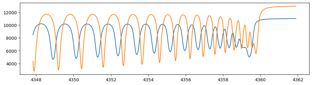
Let’s verify that spectra are being generated from fspec with
various parameter sets.
fig = plt.figure(figsize=(12, 3))

plt.plot(nu_obs, fspec(1200.0, 0.09, 0.01, gravity_jupiter(1.0, 1.0), 40.0, 10.0),label="model")
plt.plot(nu_obs, fspec(1100.0, 0.12, 0.01, gravity_jupiter(1.0, 10.0), 20.0, 5.0),label="model")
[<matplotlib.lines.Line2D at 0x719f7c1aaef0>]
NumPyro is a probabilistic programming language (PPL), which requires
the definition of a probabilistic model. In the probabilistic model
model_prob defined below, the prior distributions of each parameter
are specified. The previously defined spectral model is used within this
probabilistic model as a function that provides the mean \(\mu\).
The spectrum is assumed to be generated according to a Gaussian
distribution with this mean and a standard deviation \(\sigma\).
i.e. \(f(\nu_i) \sim \mathcal{N}(\mu(\nu_i; {\bf p}), \sigma^2 I)\),
where \({\bf p}\) is the spectral model parameter set, which are the
arguments of fspec.
import numpyro.distributions as dist
import numpyro
from jax import random
def model_prob(spectrum):

    #atmospheric/spectral model parameters priors
    logg = numpyro.sample('logg', dist.Uniform(4.0, 5.0))
    RV = numpyro.sample('RV', dist.Uniform(35.0, 45.0))
    mmr = numpyro.sample('MMR', dist.Uniform(0.0, 0.015))
    T0 = numpyro.sample('T0', dist.Uniform(1000.0, 1500.0))
    alpha = numpyro.sample('alpha', dist.Uniform(0.05, 0.2))
    vsini = numpyro.sample('vsini', dist.Uniform(5.0, 15.0))
    mu = fspec(T0, alpha, mmr, 10**logg, RV, vsini)

    #noise model parameters priors
    sigmain = numpyro.sample('sigmain', dist.Exponential(1.e-3))
    numpyro.sample('spectrum', dist.Normal(mu, sigmain), obs=spectrum)
Here, we perform retrieval using Stochastic Variational Inference (SVI) with NumPyro.
from numpyro.infer import SVI
from numpyro.infer import Trace_ELBO
import numpyro.optim as optim
In variational inference, inference is performed using a guide distribution that is computationally convenient. In many cases, designing this guide distribution is crucial, but for complex models, it can be time-consuming and challenging to find an optimal form. While it is possible to manually define a guide distribution (approximate posterior) when performing variational inference (VI), here we will use Automatic Guide Generation, which automatically generates an appropriate guide distribution based on the structure of the model.
5.1 Auto Guide using Multivariate Normal
First, let’s try an example using a multivariate normal distribution.
from numpyro.infer.autoguide import AutoMultivariateNormal
guide = AutoMultivariateNormal(model_prob)
optimizer = optim.Adam(0.01)
svi = SVI(model_prob, guide, optimizer, loss=Trace_ELBO())
SVI is generally characterized by its lower computational cost compared to HMC-NUTS or nested sampling. The execution time below should be within one minute, or at most a few minutes.
num_steps = 2000
rng_key = random.PRNGKey(0)
rng_key, rng_key_run = random.split(rng_key)
svi_result = svi.run(rng_key_run, num_steps, spectrum=Fobs)
100%|██████████| 2000/2000 [02:20<00:00, 14.21it/s, init loss: 2643771812.8775, avg. loss [1901-2000]: 616551.0235]
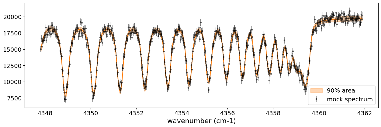
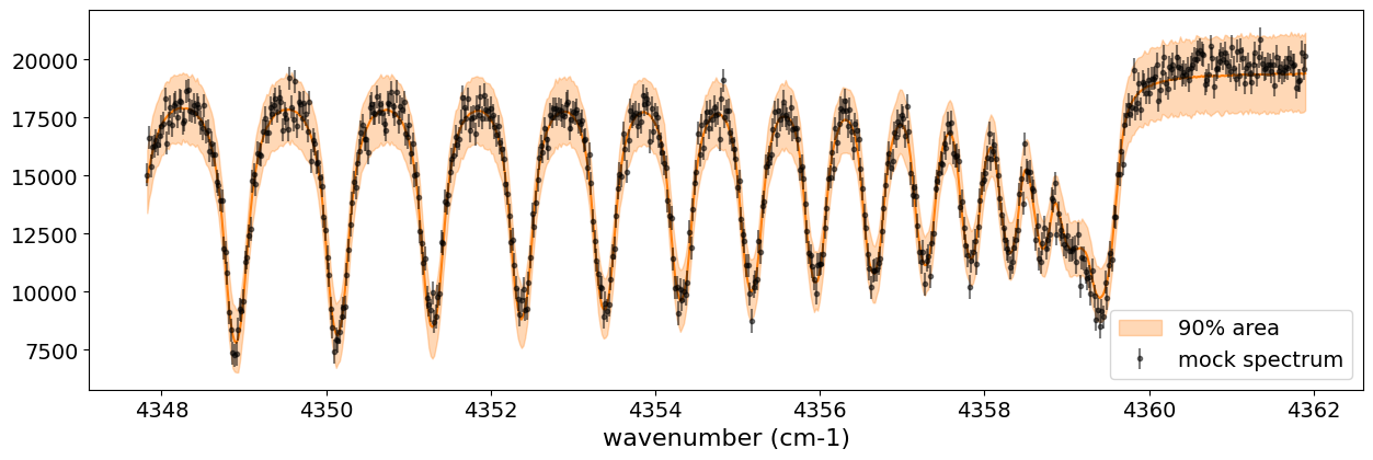
Let’s use Predictive to generate spectrum predictions and check the
results.
from numpyro.diagnostics import hpdi
from numpyro.infer import Predictive
import jax.numpy as jnp
params = svi_result.params
predictive = Predictive(
    model_prob,
    guide=guide,
    params=params,
    num_samples=2000,
    return_sites=("spectrum",),
)
predictions = predictive(rng_key, spectrum=None)
median_mu1 = jnp.median(predictions["spectrum"], axis=0)
hpdi_mu1 = hpdi(predictions["spectrum"], 0.9)
fig, ax = plt.subplots(nrows=1, ncols=1, figsize=(15, 4.5))
ax.plot(nu_obs, median_mu1, color='C1')
ax.fill_between(nu_obs,
                hpdi_mu1[0],
                hpdi_mu1[1],
                alpha=0.3,
                interpolate=True,
                color='C1',
                label='90% area')
ax.errorbar(nu_obs, Fobs, noise, fmt=".", label="mock spectrum", color="black",alpha=0.5)
plt.xlabel('wavenumber (cm-1)', fontsize=16)
plt.legend(fontsize=14)
plt.tick_params(labelsize=14)
plt.show()
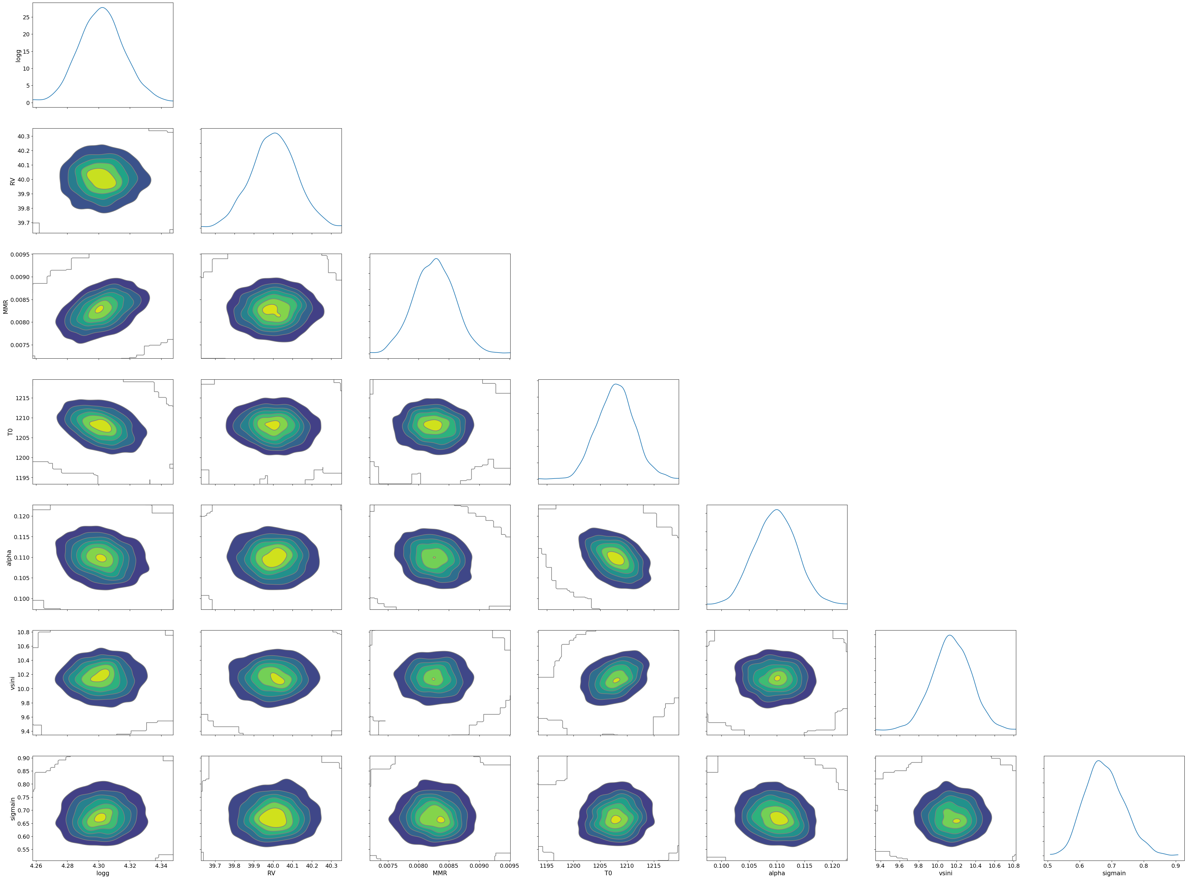
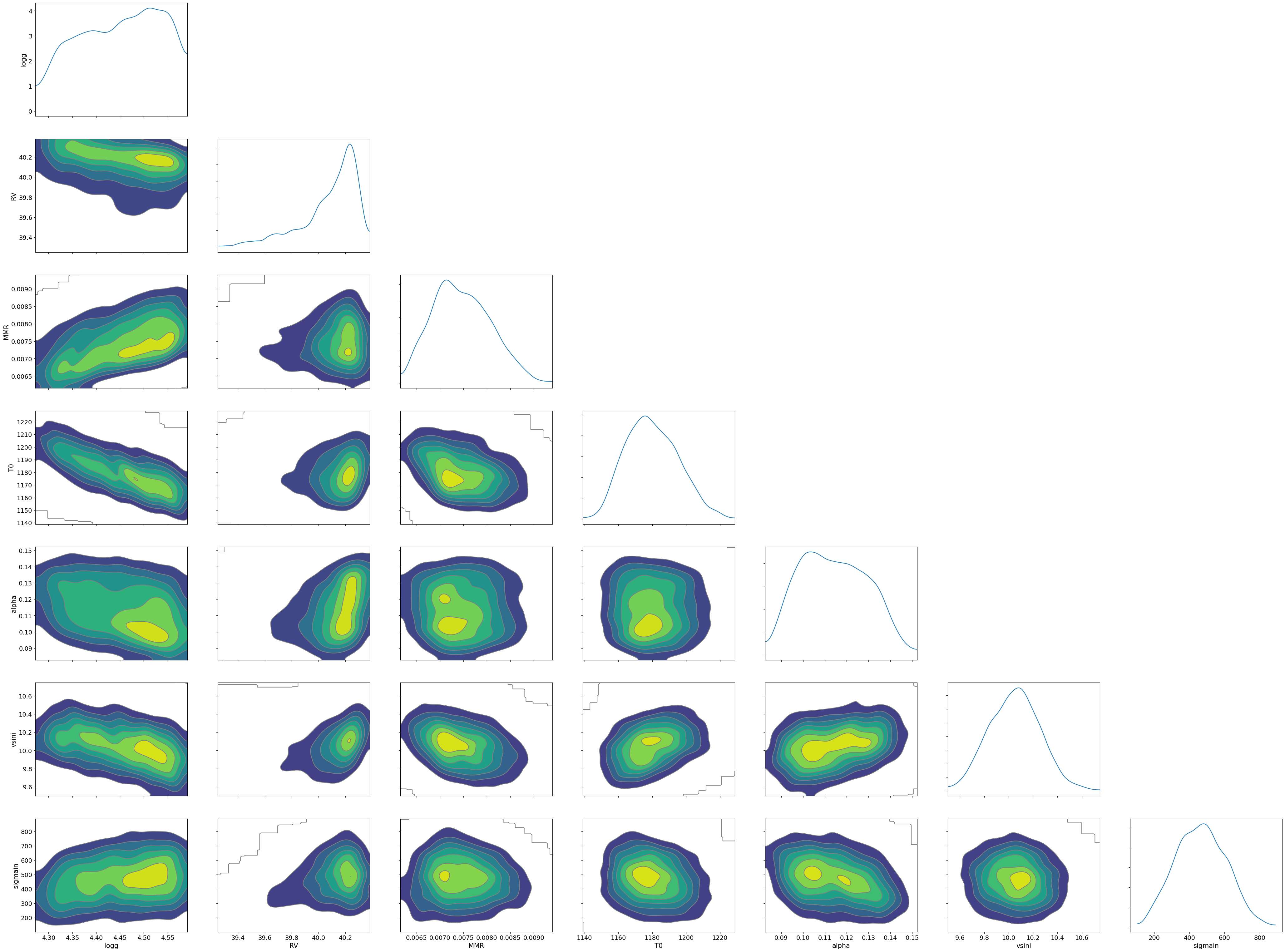
To sample parameters, you need to set the return_sites argument in
Predictive.
param_entries = ("logg", "RV", "MMR", "T0", "alpha", "vsini", "sigmain")
predictive_posterior = Predictive(
    model_prob,
    guide=guide,
    params=params,
    num_samples=2000,
    return_sites=param_entries,
)
posterior_sample = predictive_posterior(rng_key, spectrum=None)
import arviz
idata = arviz.from_dict(posterior=posterior_sample)

arviz.plot_pair(
    idata,
    var_names=param_entries,
    kind="kde",
    marginals=True,
)
plt.show()
5.2 Auto Guide for BNAF
As another example, let’s try AutoBNAFNormal, which utilizes Block
Neural Autoregressive Flow (BNAF) within the framework of normalizing
flows, a class of invertible transformations using neural networks. This
method is more flexible than standard mean-field approximations,
allowing it to capture high-dimensional and complex dependencies between
latent variables.
from numpyro.infer.autoguide import AutoBNAFNormal
guide = AutoBNAFNormal(model_prob)
optimizer = optim.Adam(0.01)
svi = SVI(model_prob, guide, optimizer, loss=Trace_ELBO())
num_steps = 10000
rng_key = random.PRNGKey(0)
rng_key, rng_key_run = random.split(rng_key)
svi_result = svi.run(rng_key_run, num_steps, spectrum=Fobs)
100%|██████████| 10000/10000 [01:10<00:00, 142.20it/s, init loss: 2630039212.8949, avg. loss [9501-10000]: 6351.8862]
params = svi_result.params
predictive = Predictive(
    model_prob,
    guide=guide,
    params=params,
    num_samples=2000,
    return_sites=("spectrum",),
)
predictions = predictive(rng_key, spectrum=None)
median_mu1 = jnp.median(predictions["spectrum"], axis=0)
hpdi_mu1 = hpdi(predictions["spectrum"], 0.9)
fig, ax = plt.subplots(nrows=1, ncols=1, figsize=(15, 4.5))
ax.plot(nu_obs, median_mu1, color='C1')
ax.fill_between(nu_obs,
                hpdi_mu1[0],
                hpdi_mu1[1],
                alpha=0.3,
                interpolate=True,
                color='C1',
                label='90% area')
ax.errorbar(nu_obs, Fobs, noise, fmt=".", label="mock spectrum", color="black",alpha=0.5)
plt.xlabel('wavenumber (cm-1)', fontsize=16)
plt.legend(fontsize=14)
plt.tick_params(labelsize=14)
plt.show()
predictive_posterior = Predictive(
    model_prob,
    guide=guide,
    params=params,
    num_samples=2000,
    return_sites=param_entries,
)
posterior_sample = predictive_posterior(rng_key, spectrum=None)
import arviz
idata = arviz.from_dict(posterior=posterior_sample)

arviz.plot_pair(
    idata,
    var_names=param_entries,
    kind="kde",
    marginals=True,
)
plt.show()
Various other Automatic Guide Generation, are also available, so explore them.
That’s it!