Why Differentiable Spectral Modeling?

Last Update: Febrary 4th (2025) Hajime Kawahara

ExoJAX is a differentiable spectral model written in JAX. Here, we aim to provide a brief introduction to what can be achieved with differentiable models for users who may not be familiar with Differentiable Programming (DP).

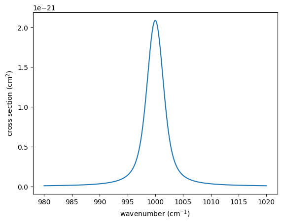
Here, as the simplest example of a spectrum, we use an absorption spectrum consisting of a single hypothetical absorption line of a molecule X. This absorption line follows a Voigt profile, characterized by a line profile centered at nu0 , determined by the temperature-dependent core width beta and the temperature- and pressure-dependent wing width gamma . The cross-section is given as follows:

import jax.numpy as jnp
import matplotlib.pyplot as plt
from exojax.spec import voigt

logbeta = 1.0
gamma = 1.0
line_strength = 1.e-20 #cm2
nu0 = 1000.0
nu_grid = jnp.linspace(nu0-20,nu0+20,1000)

sigma = line_strength*voigt(nu_grid - nu0,logbeta,gamma)

plt.plot(nu_grid, sigma)
plt.xlabel("wavenumber (cm$^{-1}$)")
plt.ylabel("cross section (cm$^2$)")

Text(0, 0.5, 'cross section (cm$^2$)')

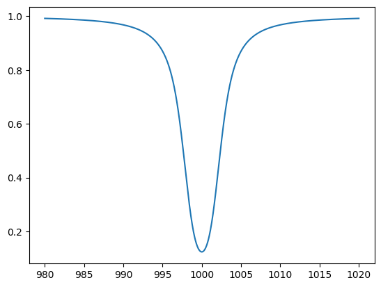
When light with a flat spectrum \(f_0\) passes through a region filled with molecule X at a number density \(n\) over a path length \(L\), the transmitted spectrum is given by \(f_0 \exp(-\tau_\nu)\), where the optical depth \(\tau_\nu = n L \sigma_\nu\). Using the column density \(N = n L\), this can be expressed as \(f_\nu = f_0 \exp{(-N \sigma_\nu )}\).

f0 = jnp.ones_like(nu_grid)
n = 1.e17
L = 1.e4
logN = n*L
f = f0*jnp.exp(-sigma*logN)

plt.plot(nu_grid, f)
plt.show()

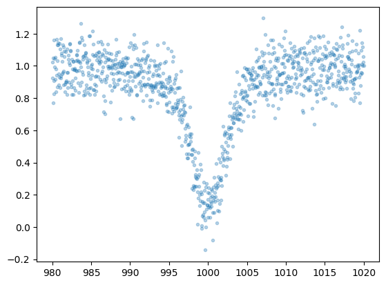
Observed spectra always contain statistical errors. Here, we simplify by assuming wavenumber-independent Gaussian noise and add noise accordingly.

import numpy as np
sigma_noise = 0.1
np.random.seed(72)
fobs = f + np.random.normal(0.0,sigma_noise,len(f))
plt.plot(nu_grid, fobs, ".",alpha=0.3)
plt.show()

Now, what can a differentiable spectral model do with this observed spectrum? Let’s first assume that gamma is known and focus on estimating N and beta.

def fmodel(N,beta):
    gamma=1.0
    nu0 = 1000.0
    sigma = line_strength*voigt(nu_grid - nu0,beta,gamma)
    f = f0*jnp.exp(-sigma*N)
    return f

Gradient-based Optimization

In a differentiable spectral model, gradient-based optimization is possible. Specifically, when \(\chi^2\) is expressed as a function of N (normalized by 1e21) and beta, we can compute the gradients of \(\chi^2\) with respect to N and beta. This allows us to determine the next step that minimizes \(\chi^2\), following the same principle as descending along the slope of a hill toward the valley bottom.

def chi2_fmodel(params):
    """differentiable chi2 function
    Args:
        params: logN (float), log surface density, logbeta (float), log beta

    Returns:
        float: chi2
    """
    logN, logbeta = params
    f = fmodel(10**logN,10**logbeta)
    return jnp.sum((f-fobs)**2/sigma_noise**2)

Here, let’s first check the distribution of \(\chi^2\). However, this is only feasible because the parameter space is two-dimensional in this case. In general, such an approach would be challenging.

Narray = jnp.linspace(20.5, 21.5, 100)
betaarray = jnp.linspace(-1, 1, 100)


# unpacks parameters
def chi2_fmodel_unpackpar(logN, logbeta):
    return chi2_fmodel(jnp.array([logN, logbeta]))


from jax import vmap

vmapchi2 = vmap(vmap(chi2_fmodel_unpackpar, (0, None), 0), (None, 0), 0)
chi2arr = vmapchi2(Narray, betaarray)

a = plt.imshow(
    chi2arr[::-1, :],
    extent=(Narray[0], Narray[-1], betaarray[0], betaarray[-1]),
    aspect="auto",
    cmap="cividis",
    vmin=1000,
    vmax=1800,
)
cb = plt.colorbar(a)
levels = [1000, 1200, 1400, 1600, 1800, 2000]
plt.contour(Narray, betaarray, chi2arr, levels=levels, colors="white")
plt.xlabel("log N")
plt.ylabel("log beta")

Text(0, 0.5, 'log beta')

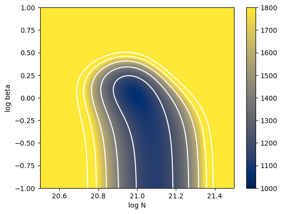
The key point here is that the \(\chi^2\) defined using a differentiable spectral model is itself differentiable with respect to the parameters.

from jax import grad
dchi2 = grad(chi2_fmodel)
logNinit = 20.75
logbetainit = 0.5
params_init = jnp.array([logNinit,logbetainit])
dchi2(params_init)

Array([-5261.481 ,  4553.8516], dtype=float32)

Let’s perform gradient-based optimization using the (differentiable) \(\chi^2\) as the cost function. The simplest gradient optimization method, steepest gradient descent, starts from an initial value and updates the parameters in the negative gradient direction. The step size \(\eta\) determines the magnitude of each update step.

\({\bf p}_n = {\bf p}_{n-1} - \eta \left( \frac{ d {\bf \chi^2}}{d {\bf p}} \right)_{n-1}\)

eta = 1.e-5
Nstep = 30
params = jnp.copy(params_init)
trajectory = []
for i in range(Nstep):
    trajectory.append(params)
    params = params - eta*dchi2(params)

trajectory = jnp.array(trajectory)

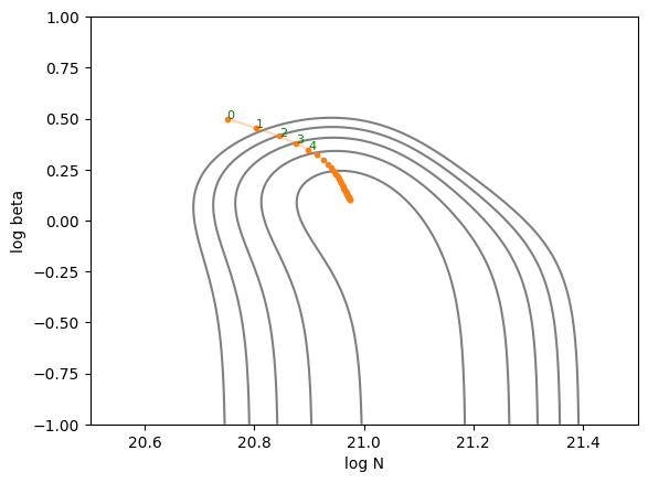
Let’s plot the trajectory of parameter updates using the steepest gradient descent method. You can observe the parameters being updated toward the local minimum. It’s interesting to experiment with different values of \(\eta\). If \(\eta\) is too large, the updates overshoot and oscillate across the valley, while if it’s too small, the descent toward the minimum becomes very slow. However, with an appropriate step size, the optimization proceeds efficiently.

def plot_trajectory(trajectory):
    plt.contour(
    Narray,
    betaarray,
    chi2arr,
    levels=levels,
    colors="gray",
)
    plt.xlabel("log N")
    plt.ylabel("log beta")
    plt.plot(trajectory[:, 0], trajectory[:, 1], ".", color="C1")
    plt.plot(trajectory[:, 0], trajectory[:, 1], color="C1", alpha=0.3)
    for i in range(5):
        plt.text(trajectory[i, 0], trajectory[i, 1], str(i), fontsize=8, color="green")

plot_trajectory(trajectory)

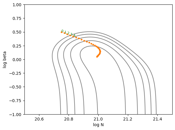
In JAX, various gradient optimization techniques can be easily implemented using Optax. Here, we’ll use one of the commonly used optimizers, ADAM, to find the parameters that minimize (or more precisely, locally minimize) \(\chi^2\).

import optax

solver = optax.adam(learning_rate=0.02)
opt_state = solver.init(params_init)
Nstep = 30
params = jnp.copy(params_init)

trajectory_adam = []
for i in range(Nstep):
    trajectory_adam.append(params)
    grad = dchi2(params)
    updates, opt_state = solver.update(grad, opt_state, params)
    params = optax.apply_updates(params, updates)

plot_trajectory(jnp.array(trajectory_adam))

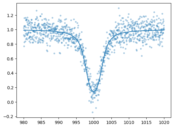
Using the updated parameters to predict the spectrum results in the following:

plt.plot(nu_grid, fobs, ".", alpha=0.3)
plt.plot(nu_grid, fmodel(10**params[0],10**params[1]), color="C0")
plt.show()

MCMC sampling using HMC-NUTS

Formal Explanation of HMC-NUTS

Hamiltonian Monte Carlo (HMC) is a Markov Chain Monte Carlo (MCMC) technique designed to efficiently sample from complex posterior distributions, often encountered in Bayesian inference. Unlike simpler methods such as Metropolis-Hastings or Gibbs sampling, HMC leverages concepts from physics, specifically Hamiltonian dynamics, to guide the sampling process. By introducing an auxiliary momentum variable and simulating the system’s energy-conserving trajectories, HMC is able to make larger, more informed proposals in the parameter space, thereby reducing the autocorrelation in the samples and improving the overall efficiency. This can be particularly helpful in high-dimensional inference problems common in astronomy (e.g., inferring orbital parameters of multiple exoplanets), where naive random-walk behavior can lead to very slow convergence.

The No-U-Turn Sampler (NUTS) is an extension of HMC that addresses a practical challenge: choosing the trajectory length (i.e., how long the Hamiltonian system is simulated before making a new proposal). Picking this length by hand can be difficult and problem-dependent. NUTS automatically determines how far to run the Hamiltonian dynamics in each iteration by building a balanced tree of possible trajectories and stopping when it detects a “U-turn” in the parameter space, indicating that further exploration would start retracing its path. This adaptation helps ensure that you sample efficiently without requiring manual tuning of trajectory lengths. In practice, many modern Bayesian software packages (like Stan, PyMC, and Numpyro) implement NUTS by default, which makes it widely accessible for astronomers who need robust sampling methods for their complex models.

The formal explanation of HMC-NUTS above was generated by ChatGPT o1 (sorry)! In essence, HMC-NUTS is the de facto standard MCMC method in Bayesian statistics. To sample using HMC-NUTS, the model must be differentiable, and the models we’ve written so far are, of course, differentiable. To apply HMC-NUTS to models written in JAX, libraries such as NumPyro and BlackJAX can be used. Here, we’ll use NumPyro.

from numpyro.infer import MCMC, NUTS
import numpyro
import numpyro.distributions as dist
from jax import random

def model(y):
    logN = numpyro.sample('logN', dist.Uniform(20.5, 21.5))
    logbeta = numpyro.sample('logbeta', dist.Uniform(-1, 1))
    sigmain = numpyro.sample('sigmain', dist.Exponential(10.0))
    N = 10**logN
    beta = 10**logbeta
    mu = fmodel(N,beta)
    numpyro.sample('y', dist.Normal(mu, sigmain), obs=y)

rng_key = random.PRNGKey(0)
rng_key, rng_key_ = random.split(rng_key)
num_warmup, num_samples = 1000, 2000
kernel = NUTS(model)
mcmc = MCMC(kernel, num_warmup=num_warmup, num_samples=num_samples)
mcmc.run(rng_key_, y=fobs)
mcmc.print_summary()

sample: 100%|██████████| 3000/3000 [00:08<00:00, 361.90it/s, 3 steps of size 6.79e-01. acc. prob=0.91]

                mean       std    median      5.0%     95.0%     n_eff     r_hat
      logN     20.99      0.01     20.99     20.97     21.01   1217.43      1.00
   logbeta      0.01      0.03      0.02     -0.03      0.06   1406.41      1.00
   sigmain      0.10      0.00      0.10      0.10      0.11   1592.57      1.00

Number of divergences: 0

import arviz
from numpyro.diagnostics import hpdi
from numpyro.infer import Predictive

# SAMPLING
posterior_sample = mcmc.get_samples()
pred = Predictive(model, posterior_sample, return_sites=['y'])
predictions = pred(rng_key_, y=None)
median_mu1 = jnp.median(predictions['y'], axis=0)
hpdi_mu1 = hpdi(predictions['y'], 0.9)

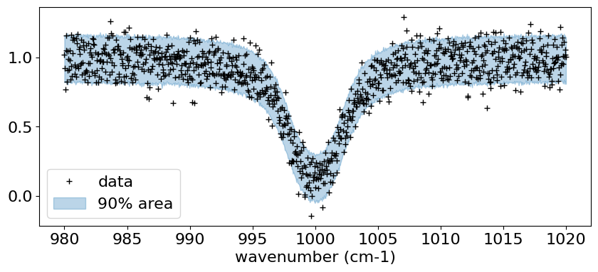
# PLOT
fig, ax = plt.subplots(nrows=1, ncols=1, figsize=(10, 4))
#ax.plot(nu_grid, median_mu1, color='C0')
ax.plot(nu_grid, fobs, '+', color='black', label='data')
ax.fill_between(nu_grid,
                hpdi_mu1[0],
                hpdi_mu1[1],
                alpha=0.3,
                interpolate=True,
                color='C0',
                label='90% area')

plt.xlabel('wavenumber (cm-1)', fontsize=16)
plt.legend(fontsize=16)
plt.tick_params(labelsize=16)
plt.show()

pararr = ["logN", "logbeta", "sigmain"]
arviz.plot_pair(
    arviz.from_numpyro(mcmc),
    kind="kde",
    divergences=False,
    marginals=True,
    reference_values={"logN": 21.0, "logbeta": 0.0, "sigmain": 0.1},
)

array([[<Axes: ylabel='logN'>, <Axes: >, <Axes: >],
       [<Axes: ylabel='logbeta'>, <Axes: >, <Axes: >],
       [<Axes: xlabel='logN', ylabel='sigmain'>,
        <Axes: xlabel='logbeta'>, <Axes: xlabel='sigmain'>]], dtype=object)

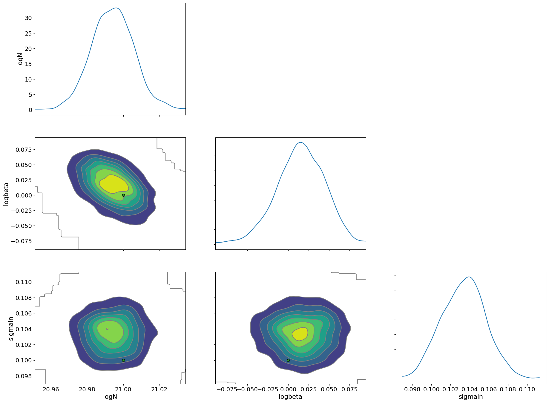
Here, we used a simple absorption line spectrum, so the HMC execution time should be within a few seconds to a few minutes. ExoJAX can compute emission spectra, reflection spectra, and transmission spectra from atmospheric layers, all of which are differentiable and can be used for Bayesian analysis with HMC, just like in this example.

For more details, please start by referring to Getting Started Guide.

When the model is differentiable, inference methods other than HMC that utilize gradients are also possible. Next, as an example, let’s try Stochastic Variational Inference (SVI).

from numpyro.infer import SVI
from numpyro.infer import Trace_ELBO
import numpyro.optim as optim
from numpyro.infer.autoguide import AutoMultivariateNormal

guide = AutoMultivariateNormal(model)
optimizer = optim.Adam(0.01)
svi = SVI(model, guide, optimizer, loss=Trace_ELBO())

SVI is faster compared to HMC.

num_steps = 10000
rng_key = random.PRNGKey(0)
rng_key, rng_key_run = random.split(rng_key)
svi_result = svi.run(rng_key_run, num_steps, y=fobs)

100%|██████████| 10000/10000 [00:04<00:00, 2037.36it/s, init loss: -102.3971, avg. loss [9501-10000]: -840.5520]

params = svi_result.params
predictive_posterior = Predictive(
    model,
    guide=guide,
    params=params,
    num_samples=2000,
    return_sites=pararr,
)
posterior_sample = predictive_posterior(rng_key, y=None)

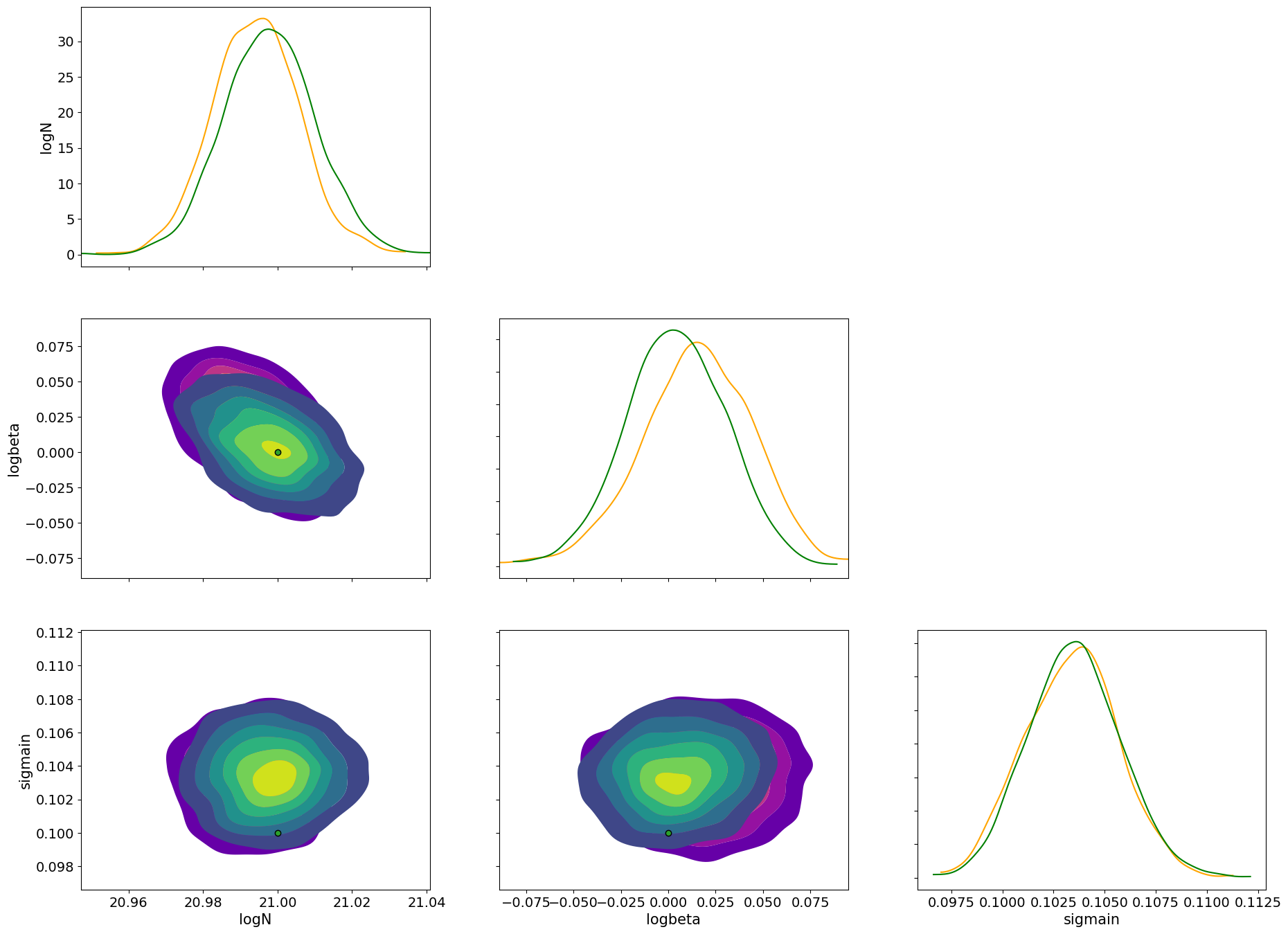
Let’s compare the posterior distributions of HMC (orange) and SVI (green).

import arviz
idata = arviz.from_dict(posterior=posterior_sample)

axes = arviz.plot_pair(
    arviz.from_numpyro(mcmc),
    var_names=pararr,
    kind="kde",
    marginals=True,
    show=False,
    kde_kwargs={"contourf_kwargs":{"cmap":"plasma","alpha":0.5},"contour_kwargs":{"alpha":0}},
    marginal_kwargs={"color":"orange"},
)
axes2 = arviz.plot_pair(
    idata,
    ax = axes,
    var_names=pararr,
    kind="kde",
    marginals=True,
    show=False,
    reference_values={"logN": 21.0, "logbeta": 0.0, "sigmain": 0.1},
    kde_kwargs={"contourf_kwargs":{"alpha":0.5,"cmap":"viridis"}, "contour_kwargs":{"alpha":0}},
    marginal_kwargs={"color":"green"}
)
plt.show()

Please refer to the SVI getting started guide.

Here, we introduced both HMC and SVI, but inference methods that do not rely on differentiation, such as Nested Sampling, are also efficient thanks to JAX’s XLA acceleration. See this guide for more details.

Conclusion

In summary, differentiable models greatly expand the possibilities for retrieval inference!