Voigt-Hjerting Function and Voigt Profile

Update: May 21/2021, Hajime Kawahara

Voigt-Hjerting Function

The Voigt-Hjerting function is the real part of the Faddeeva function, defined as

\(H(x,a) = \frac{a}{\pi}\) \(\int_{-\infty}^{\infty}\) \(\frac{e^{-y^2}}{(x-y)^2 + a^2} dy\) .

In exojax, hjert provides the Voigt-Hjerting function.

from exojax.spec import hjert
hjert(1.0,1.0)

DeviceArray(0.3047442, dtype=float32)

We can differentiate the Voigt-Hjerting function by \(x\). \(\partial_x H(x,a)\) is given by

from jax import grad
dhjert_dx=grad(hjert,argnums=0)
dhjert_dx(1.0,1.0)

DeviceArray(-0.1930505, dtype=float32)

hjert is compatible to JAX. So, when you want to use array as input, you need to wrap it by jax.vmap.

import jax.numpy as jnp
from jax import vmap
import matplotlib.pyplot as plt

#input vector
x=jnp.linspace(-5,5,100)

#vectorized hjert H(x,a)
vhjert=vmap(hjert,(0,None),0)

#vectroized dH(x,a)/dx
vdhjert_dx=vmap(dhjert_dx,(0,None),0)

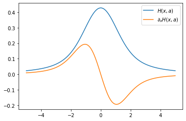
plt.plot(x, vhjert(x,1.0),label="$H(x,a)$")
plt.plot(x, vdhjert_dx(x,1.0),label="$\\partial_x H(x,a)$")
plt.legend()

Voigt Profile

Using the Voigt-Hjerting function, the Voigt profile is expressed as

\(V(\nu, \beta, \gamma_L) = \frac{1}{\sqrt{2 \pi} \beta} H\left( \frac{\nu}{\sqrt{2} \beta},\frac{\gamma_L}{\sqrt{2} \beta} \right)\)

\(V(\nu, \beta, \gamma_L)\) is a convolution of a Gaussian with a STD of \(\beta\) and a Lorentian with a gamma parameter of \(\gamma_L\).

from exojax.spec import voigt
import jax.numpy as jnp
import matplotlib.pyplot as plt

nu=jnp.linspace(-10,10,100)
plt.plot(nu, voigt(nu,1.0,2.0)) #beta=1.0, gamma_L=2.0

See ” Voigt profile ” for the tutorial of the Voigt profile.