Voigt profile

from exojax.spec import voigt
import jax.numpy as jnp
import matplotlib.pyplot as plt

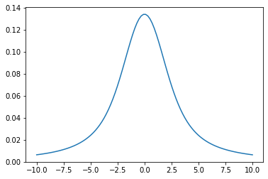
Let’s compute the Voigt function $V(\nu, \beta, \gamma_L)$ using exojax! $V(\nu, \beta, \gamma_L)$ is a convolution of a Gaussian with a STD of $\beta$ and a Lorentian with a gamma parameter of $\gamma_L$.

nu=jnp.linspace(-10,10,100)
plt.plot(nu, voigt(nu,1.0,2.0)) #beta=1.0, gamma_L=2.0

[<matplotlib.lines.Line2D at 0x7faaf9d64358>]

The function “voigt” is vmapped for nu (input=0), therefore a bit hard to handle when you want to differentiate. Instead, you can use “voigtone”, which is not vmapped for all of the input arguments.

from exojax.spec import voigtone
from jax import grad, vmap

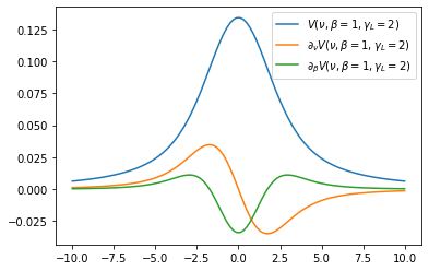
dvoigt_nu=vmap(grad(voigtone,argnums=0),(0,None,None),0) #derivative by nu
dvoigt_beta=vmap(grad(voigtone,argnums=1),(0,None,None),0) #derivative by beta

plt.plot(nu, voigt(nu,1.0,2.0),label="$V(\\nu,\\beta=1,\\gamma_L=2)$")
plt.plot(nu, dvoigt_nu(nu,1.0,2.0),label="$\\partial_\\nu V(\\nu,\\beta=1,\\gamma_L=2)$")
plt.plot(nu, dvoigt_beta(nu,1.0,2.0),label="$\\partial_\\beta V(\\nu,\\beta=1,\\gamma_L=2)$")
plt.legend()

<matplotlib.legend.Legend at 0x7faaf9b45c50>

HMC-NUTS of a simple absorption model

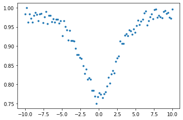
Next, we try to fit a simple absorption model to mock data. The absorption model is

$ e^{-a V(:raw-latex:`\nu`,:raw-latex:beta,:raw-latex:gamma_L)}$

def absmodel(nu,a,beta,gamma_L):
    return jnp.exp(-a*voigt(nu,beta,gamma_L))

Adding a noise…

from numpy.random import normal
data=absmodel(nu,2.0,1.0,2.0)+normal(0.0,0.01,len(nu))
plt.plot(nu,data,".")

[<matplotlib.lines.Line2D at 0x7faaf97f9710>]

Then, let’s perfomr a HMC-NUTS.

import arviz
import numpyro.distributions as dist
import numpyro
from numpyro.infer import MCMC, NUTS
from numpyro.infer import Predictive
from numpyro.diagnostics import hpdi

def model_c(nu,y):
    sigma = numpyro.sample('sigma', dist.Exponential(1.0))
    a = numpyro.sample('a', dist.Exponential(1.0))
    beta = numpyro.sample('beta', dist.Exponential(1.0))
    gamma_L = numpyro.sample('gammaL', dist.Exponential(1.0))
    mu=absmodel(nu,a,beta,gamma_L)
    numpyro.sample('y', dist.Normal(mu, sigma), obs=y)

from jax import random
rng_key = random.PRNGKey(0)
rng_key, rng_key_ = random.split(rng_key)
num_warmup, num_samples = 1000, 2000

kernel = NUTS(model_c,forward_mode_differentiation=True)
mcmc = MCMC(kernel, num_warmup, num_samples)
mcmc.run(rng_key_, nu=nu, y=data)

sample: 100%|██████████| 3000/3000 [00:48<00:00, 65.47it/s, 15 steps of size 1.93e-01. acc. prob=0.95]

posterior_sample = mcmc.get_samples()
pred = Predictive(model_c,posterior_sample)
predictions = pred(rng_key_,nu=nu,y=None)

median_mu = jnp.median(predictions["y"],axis=0)
hpdi_mu = hpdi(predictions["y"], 0.9)

fig, ax = plt.subplots(nrows=1, ncols=1)
ax.plot(nu,median_mu,color="C0")
ax.plot(nu,data,"+",color="C1",label="data")
ax.fill_between(nu, hpdi_mu[0], hpdi_mu[1], alpha=0.3, interpolate=True,color="C0",
                label="90% area")
plt.xlabel("$\\nu$",fontsize=16)
plt.legend()

<matplotlib.legend.Legend at 0x7faa2408aa20>

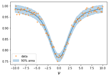
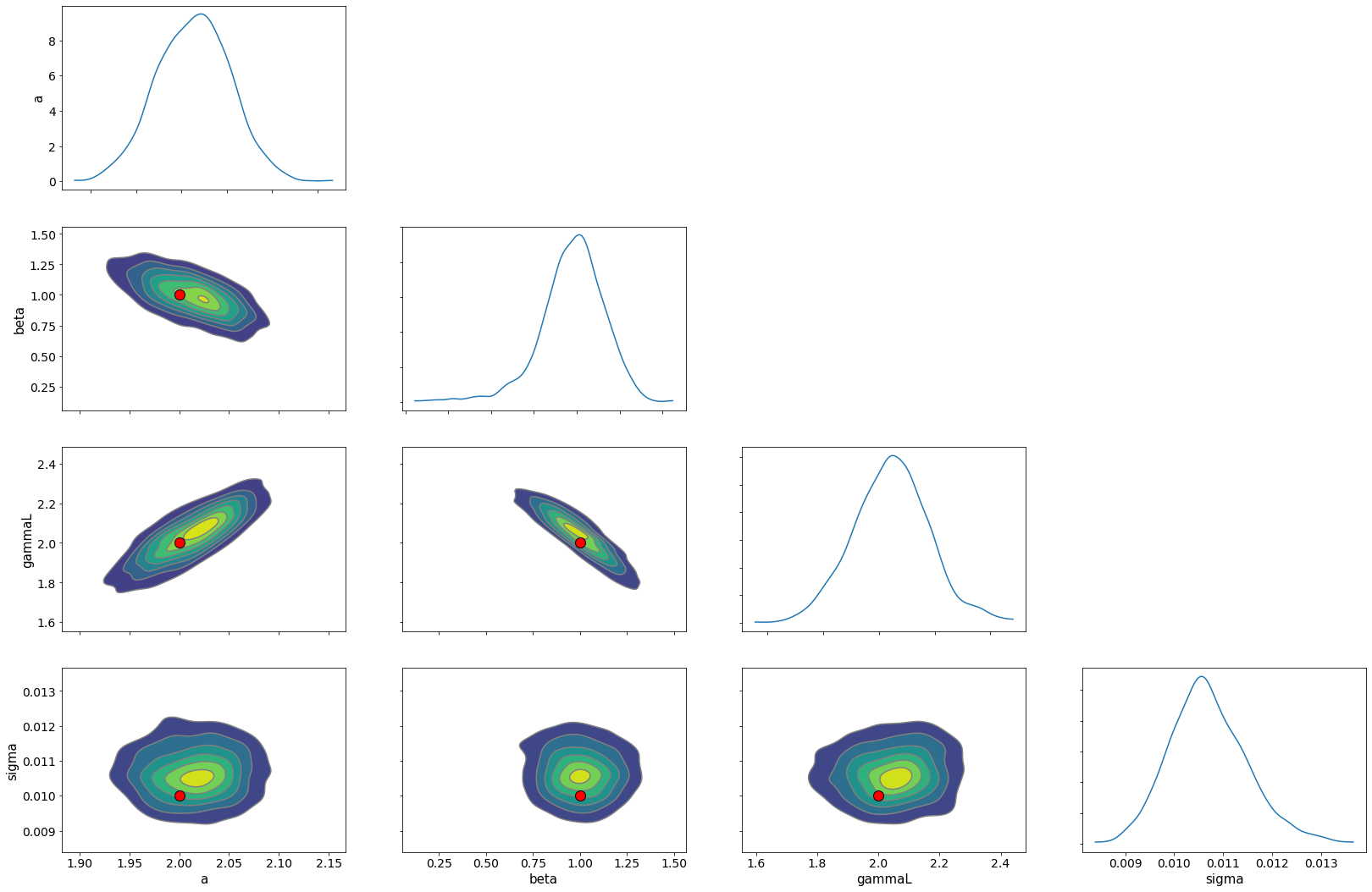
We got a posterior sampling.

refs={};refs["sigma"]=0.01;refs["a"]=2.0;refs["beta"]=1.0;refs["gammaL"]=2.0
arviz.plot_pair(arviz.from_numpyro(mcmc),kind='kde',\
                divergences=False,marginals=True,reference_values=refs,\
               reference_values_kwargs={'color':"red", "marker":"o", "markersize":12})
plt.show()

curve of growth

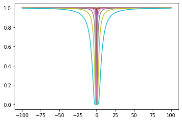
As an application, we consider the curve of growth. The curve of growth is the equivalent width evolution as a function of the absorption sterngth. Here, it corresponds to $a$. Let’s see, the growth of absorption feature as

nu=jnp.linspace(-100,100,10000)
aarr=jnp.logspace(-3,3,10)
for a in aarr:
    plt.plot(nu,absmodel(nu,a,0.1,0.1))

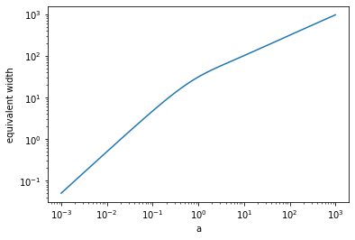
Let us define the equivalent width by a simple summation of the absorption.

def EW(a):
    return jnp.sum(1-absmodel(nu,a,0.1,0.1))
vEW=vmap(EW,0,0)

This is the curve of growth. As you see, when the absorption is weak, the power of the curve is proportional to unity (linear region). But, as increasing the absorption sterength, the power converges to 1/2.

aarr=jnp.logspace(-3,3,100)
plt.plot(aarr,vEW(aarr))
plt.yscale("log")
plt.xscale("log")
plt.xlabel("a")
plt.ylabel("equivalent width")
plt.show()

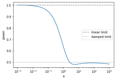
Now we have auto-diff for the Voigt. So, we can directly compute the power as a function of $a$.

$power = :raw-latex:`\frac{\partial}{\partial \log_{10} a }` :raw-latex:`\log`_{10} ( EW ) $

def logEW(loga):
    return jnp.log10(jnp.sum(1-absmodel(nu,10**(loga),0.1,0.1)))

dlogEW=grad(logEW)
vlogdEW=vmap(dlogEW,0,0)

logaarr=jnp.linspace(-3,3,100)
plt.plot(10**(logaarr),vlogdEW(logaarr))
plt.axhline(1.0,label="linear limit",color="gray",ls="dashed")
plt.axhline(0.5,label="damped limit",color="gray",ls="dotted")
plt.xscale("log")
plt.xlabel("a")
plt.ylabel("power")
plt.legend()
plt.show()