Foward Modeling of Jupiter-like Ammonia Clouds and Its Reflection Spectrum
Note:
To run this tutorial, you need to install PyMieScatt.
pip install PyMieScatt
See https://pymiescatt.readthedocs.io/en/latest/
import jax.numpy as jnp
import numpy as np
Sets the wavenumber range and the atmosphere model
from exojax.utils.grids import wavenumber_grid

N = 10000
nus, wav, res = wavenumber_grid(10**3, 10**4, N, xsmode="premodit")

from exojax.spec.atmrt import ArtReflectPure
from exojax.utils.astrofunc import gravity_jupiter

art = ArtReflectPure(nu_grid=nus, pressure_btm=1.0e2, pressure_top=1.0e-3, nlayer=100)
art.change_temperature_range(80.0, 400.0)
Tarr = art.powerlaw_temperature(150.0, 0.2)
Parr = art.pressure
mu = 2.3  # mean molecular weight
gravity = gravity_jupiter(1.0, 1.0)
xsmode =  premodit
xsmode assumes ESLOG in wavenumber space: mode=premodit
======================================================================
The wavenumber grid should be in ascending order.
The users can specify the order of the wavelength grid by themselves.
Your wavelength grid is in *  descending  * order
======================================================================
/home/kawahara/exojax/src/exojax/utils/grids.py:142: UserWarning: Resolution may be too small. R=4342.510524550615
  warnings.warn('Resolution may be too small. R=' + str(resolution),
/home/kawahara/exojax/src/exojax/spec/dtau_mmwl.py:14: FutureWarning: dtau_mmwl might be removed in future.
  warnings.warn("dtau_mmwl might be removed in future.", FutureWarning)
pdb is a class for particulates databases. We here use PdbCloud
for NH3, i.e. pdb for the ammonia cloud. PdbCloud uses the
refraction (refractive) indice given by VIRGA.
The precomputed grid of the Mie parameters assuming a log-normal
distribution is called miegrid. This can be computed
pdb.generate_miegrid if you do not have it. To compute miegrid, we
use PyMieScatt as a calculator.
You can also choose not to use miegrid. Instead, we compute the Mie
parameters using PyMieScatt one by one. This mode cannot be used for
the retrieval, but is useful for a one-time modeling, (a.k.a forward
modeling) of the spectrum.
Also, amp is a class for atmospheric micorphysics. AmpAmcloud is the
class for the Akerman and Marley 2001 cloud model (AM01). We adopt the
background atmosphere to hydorogen atmosphere.
from exojax.spec.pardb import PdbCloud
from exojax.atm.atmphys import AmpAmcloud

pdb_nh3 = PdbCloud("NH3")
#pdb_nh3.generate_miegrid() # when you use the miegrid
#pdb_nh3.load_miegrid() # when you use the miegrid

amp_nh3 = AmpAmcloud(pdb_nh3,bkgatm="H2")
amp_nh3.check_temperature_range(Tarr)
.database/particulates/virga/virga.zip  exists. Remove it if you wanna re-download and unzip.
Refractive index file found:  .database/particulates/virga/NH3.refrind
Miegrid file does not exist at  .database/particulates/virga/miegrid_lognorm_NH3.mg.npz
Generate miegrid file using pdb.generate_miegrid if you use Mie scattering
/home/kawahara/exojax/src/exojax/atm/atmphys.py:50: UserWarning: min temperature 80.0 K is smaller than min(vfactor t range) 179.10000610351562 K
  warnings.warn(
The substance density of the condensate is given by
condensate_substance_density. Do not confuse it with the density of
the condensates in the atmosphere.
rhoc = pdb_nh3.condensate_substance_density #g/cc
Sets the parameters in the AM01 cloud model. calc_ammodel method
computes the vertical distribution of rg and the condensate volume
mixing ratio.
from exojax.utils.zsol import nsol
from exojax.atm.mixratio import vmr2mmr
from exojax.spec.molinfo import molmass_isotope

n = nsol()  #solar abundance
abundance_nh3 = n["N"]
molmass_nh3 = molmass_isotope("NH3", db_HIT=False)

fsed = 10.
sigmag = 2.0
Kzz = 1.e4
MMRbase_nh3 = vmr2mmr(abundance_nh3, molmass_nh3, mu)

rg_layer, MMRc = amp_nh3.calc_ammodel(Parr, Tarr, mu, molmass_nh3, gravity, fsed, sigmag, Kzz, MMRbase_nh3)
The following is just to convert MMR to g/L.
from exojax.atm.idealgas import number_density
from exojax.utils.constants import m_u
fac = molmass_nh3*m_u*number_density(Parr,Tarr)*1.e3 #g/L
Plots rg, MMR, and the cloud density (g/L). Note that the cloud density agrees with Figure 2 of HU ApJ 887, 166 (2019)
import matplotlib.pyplot as plt
fig = plt.figure(figsize=(15,5))
ax = fig.add_subplot(131)
plt.plot(rg_layer,Parr)
plt.xlabel("rg (cm)")
plt.ylabel("pressure (bar)")
plt.yscale("log")
ax.invert_yaxis()
ax = fig.add_subplot(132)
plt.plot(MMRc,Parr)
plt.xlabel("condensate MMR")
plt.yscale("log")
plt.xscale("log")
plt.xlim(1e-12, 1e-2)
ax.invert_yaxis()
ax = fig.add_subplot(133)
plt.plot(fac*MMRc,Parr)
plt.xlabel("condensate density g/L")
plt.yscale("log")
plt.xscale("log")
plt.xlim(1e-8, 1e-2)
ax.invert_yaxis()
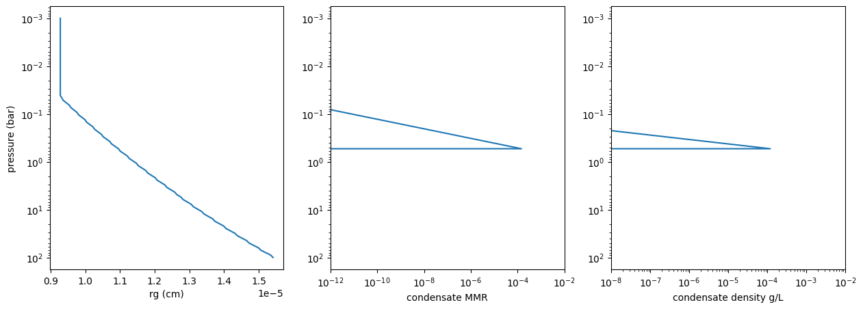
rg is almost constant through the vertical distribution. So, let’s
set a mean value here.
If you’ve already generated the miegrid, miegrid_interpolated_value
method interpolates the original parameter set given by MiQ_lognormal in
PyMieScatt. See
https://pymiescatt.readthedocs.io/en/latest/forward.html#Mie_Lognormal.
The number of the original parameters are seven, Bext, Bsca, Babs, G,
Bpr, Bback, and Bratio.
If not yet, opa.mieparams_vector_direct_from_pymiescatt directly
calls the PyMieScatt and computes the Mie parameters.
rg = 1e-5
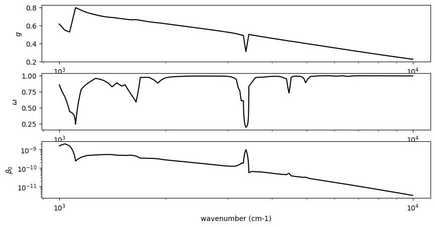
Plots the extinction coefficient for instance (index=0) and some approximation from the Kevin Heng’s textbook .
OpaMie class as
opa.mieparams_vector method,
which returns \(\beta_0\): the extinction coefficient of the
reference number density \(N_0\), \(\omega\): a single
scattering albedo , and \(g\): the asymmetric parameter.from exojax.spec.opacont import OpaMie
opa = OpaMie(pdb_nh3, nus)
#sigma_extinction, sigma_scattering, asymmetric_factor = opa.mieparams_vector(rg,sigmag) # if using MieGrid
sigma_extinction, sigma_scattering, asymmetric_factor = opa.mieparams_vector_direct_from_pymiescatt(rg, sigmag)
100%|██████████| 131/131 [00:28<00:00, 4.59it/s]
# plt.plot(pdb_nh3.refraction_index_wavenumber, miepar[50,:,0])
fig = plt.figure(figsize=(10,5))
ax = fig.add_subplot(311)
plt.plot(nus, asymmetric_factor, color="black")
plt.xscale("log")
plt.ylabel("$g$")
ax = fig.add_subplot(312)
plt.plot(nus, sigma_scattering/sigma_extinction, label="single scattering albedo", color="black")
plt.xscale("log")
plt.ylabel("$\\omega$")
ax = fig.add_subplot(313)
plt.plot(nus, sigma_extinction, label="ext", color="black")
plt.xscale("log")
plt.yscale("log")
plt.xlabel("wavenumber (cm-1)")
plt.ylabel("$\\beta_0$")
plt.savefig("miefig.png")
Reflection spectrum
The opacity of the lognormal cloud model can be computed using
opacity_profile_cloud_lognormal method in art.
dtau = art.opacity_profile_cloud_lognormal(sigma_extinction, rhoc, MMRc, rg, sigmag, gravity)
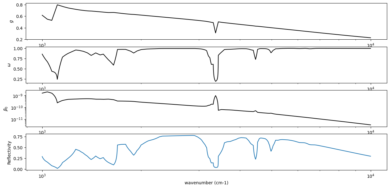
To compute the reflection spectrum, we need the single scattering albedo, asymmetric parameter (known as g, but confusing from gravity), and the surface reflectivity.
single_scattering_albedo = sigma_scattering[None,:]/sigma_extinction[None,:] + np.zeros((len(art.pressure), len(nus)))
asymmetric_parameter = asymmetric_factor + np.zeros((len(art.pressure), len(nus)))
reflectivity_surface = np.zeros(len(nus))
The incoming flux is normalized to 1. So, the output should be refelectivity.
incoming_flux = np.ones(len(nus))
Fr = art.run(dtau,single_scattering_albedo,asymmetric_parameter,reflectivity_surface,incoming_flux)
Here are the results.
fig = plt.figure(figsize=(15,7))
ax = fig.add_subplot(411)
plt.plot(nus, asymmetric_factor, color="black")
plt.xscale("log")
plt.ylabel("$g$")
ax = fig.add_subplot(412)
plt.plot(nus, sigma_scattering/sigma_extinction, label="single scattering albedo", color="black")
plt.xscale("log")
plt.ylabel("$\\omega$")
ax = fig.add_subplot(413)
plt.plot(nus, sigma_extinction, label="ext", color="black")
plt.xscale("log")
plt.yscale("log")
plt.xlabel("wavenumber (cm-1)")
plt.ylabel("$\\beta_0$")
ax = fig.add_subplot(414)
plt.plot(nus,Fr)
plt.xscale("log")
plt.ylabel("Reflectivity")
plt.xlabel("wavenumber (cm-1)")
Text(0.5, 0, 'wavenumber (cm-1)')