A wide range transmission spectrum using ExoMolOP CKD opacity

ExoMolOP provides the CKD h5 data through ExoMol website. The precomputing opacity is very handy to compute wide low resolution spectra. This tutorial shows how to compute a transmission spectrum using OpaCKD from the external opacity source, ExoMolOP.

import numpy as np
import matplotlib.pyplot as plt
from jax import config

# ExoJAX imports
from exojax.opacity import OpaCKD
from exojax.rt import ArtTransPure

# Enable 64-bit precision for accurate calculations
config.update("jax_enable_x64", True)

art = ArtTransPure(
    pressure_top=1.0e-8,
    pressure_btm=1.0e2,
    nlayer=50,  # Fewer layers for transmission calculations
    integration="simpson"  # Simpson integration for better accuracy
)

# Create atmospheric profiles
Tarr = np.linspace(1000.0, 1500.0, 50)  # Temperature profile
mmr_arr = np.full(50, 0.1)  # Constant H2O mixing ratio
mean_molecular_weight = np.full(50, 2.33)  # Mean molecular weight (H2-dominated)

# Planetary parameters (Jupiter-like)
radius_btm = 6.9e9  # Planet radius at bottom of atmosphere (cm)
gravity = 2478.57   # Surface gravity (cm/s²)

integration:  simpson
Simpson integration, uses the chord optical depth at the lower boundary and midppoint of the layers.

/home/kawahara/exojax/src/exojax/rt/common.py:40: UserWarning: nu_grid is not given. specify nu_grid when using 'run'
  warnings.warn(

Loading ExoMolOP Opacity Data

When calling OpaCKD as shown below, it automatically downloads ExoMolOP data and configures the opacity object. If you already have the data file, you can specify the file path directly instead.

nurange = [1000.0, 10000.0]
opa = OpaCKD.from_external("exomolop", ".database/CO/12C-16O/Li2015/", nurange=nurange)

#opa = OpaCKD.from_external("exomolop","12C-16O__Li2015.R1000_0.3-50mu.ktable.petitRADTRANS.h5")
#opa = OpaCKD.from_external("exomolop", ".database/CO/12C-16O/Li2015/12C-16O__Li2015.R1000_0.3-50mu.ktable.petitRADTRANS.h5")

/home/kawahara/exojax/src/exojax/utils/molname.py:197: FutureWarning: e2s will be replaced to exact_molname_exomol_to_simple_molname.
  warnings.warn(
/home/kawahara/exojax/src/exojax/utils/molname.py:91: FutureWarning: exojax.utils.molname.exact_molname_exomol_to_simple_molname will be replaced to radis.api.exomolapi.exact_molname_exomol_to_simple_molname.
  warnings.warn(

Downloading from https://www.exomol.com/db/CO/12C-16O/Li2015/12C-16O__Li2015.R1000_0.3-50mu.ktable.petitRADTRANS.h5
.database/CO/12C-16O/Li2015/12C-16O__Li2015.R1000_0.3-50mu.ktable.petitRADTRANS.h5 already exists. Skip downloading.

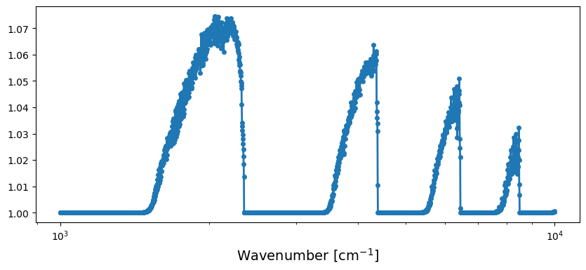
Computing a Transmission Spectra using CKD

One can compute a transmission spectrum with the following code.

xs_ckd = opa.xstensor_ckd(Tarr, art.pressure)
dtau_ckd = art.opacity_profile_xs_ckd(xs_ckd, mmr_arr, opa.molmass, gravity)
transit_ckd = art.run_ckd(dtau_ckd, Tarr, mean_molecular_weight, radius_btm, gravity, opa.ckd_info.weights)

Visualization

# Create plot
plt.figure(figsize=(10, 4))

# Plot CKD spectrum
plt.plot(opa.nu_bands, transit_ckd,
         'o-', label="CKD Method",
         markersize=4, linewidth=2, color='C0')
plt.xlabel("Wavenumber [cm$^{-1}$]", fontsize=14)
plt.xscale('log')