Comparison of the ExoJAX AM cloud model with VIRGA

March 9th in 2024, Hajime Kawahara

Here, we try to compare our cloud implementation using Ackerman and Marley Model with VIRGA. We consider the enstatite (MgSiO3) cloud.

import jax.numpy as jnp
import matplotlib.pyplot as plt
import numpy as np
import virga.justdoit as jdi

# set common values
from exojax.utils.astrofunc import gravity_jupiter
fsed = 3.0
gravity = gravity_jupiter(1.0,1.0)
mu=2.2

import virga.justplotit as jpi
import astropy.units as u
fsed = 3
miedir = "/home/kawahara/exojax/documents/tutorials/.database/particulates/virga"
#miedir = "/home/exoplanet01/exojax/documents/tutorials/.database/particulates/virga"
#miedir = "/home/exoplanet01/exojax/tests/integration/comparison/clouds/.database/particulates/virga"
a = jdi.Atmosphere(["MgSiO3"], fsed = fsed, mh=1.0, mmw=mu)
a.gravity(gravity=gravity, gravity_unit=u.Unit('cm/(s**2)'))
a.ptk(df = jdi.hot_jupiter())
all_out = jdi.compute(a, as_dict=True, directory = miedir)

pressure = all_out["pressure"]
temperature = all_out["temperature"]

#comparison w/ kawashima's vapor pressure code
def T_MgSiO3(P,metaldex):
    return 1e4 / (6.26 - 0.35 * np.log10(P) - 0.70 * metaldex) # Visscher et al. (2010)
def T_MnS(P,metaldex):
    return 1e4 / (7.447 - 0.42 * np.log10(P) - 0.84 * metaldex) # Morley et al. (2012)

Setting a simple atmopheric model. We need the density of atmosphere.

from exojax.utils.constants import kB, m_u
from exojax.atm.atmprof import pressure_layer_logspace

#Parr, dParr, k = pressure_layer_logspace(log_pressure_top=-5., log_pressure_btm=4.0, nlayer=100)
#alpha = 0.097
#T0 = 1200.
#Tarr = T0 * (Parr)**alpha

mu = 2.0  # mean molecular weight
R = kB / (mu * m_u)
rho = pressure / (R * temperature)

We import pdb as the particulate database class.

from exojax.spec.pardb import PdbCloud

pdb = PdbCloud("MgSiO3", path=miedir)
#pdb.generate_miegrid()
#pdb.load_miegrid()
#print(len(pdb.rg_arr), len(pdb.sigmag_arr))

/home/kawahara/exojax/documents/tutorials/.database/particulates/virga/virga.zip  exists. Remove it if you wanna re-download and unzip.
Refractive index file found:  /home/kawahara/exojax/documents/tutorials/.database/particulates/virga/MgSiO3.refrind
Miegrid file does not exist at  /home/kawahara/exojax/documents/tutorials/.database/particulates/virga/miegrid_lognorm_MgSiO3.mg.npz
Generate miegrid file using pdb.generate_miegrid if you use Mie scattering

The solar abundance can be obtained using utils.zsol.nsol. Here, we assume a maximum VMR for MgSiO3 from solar abundance.

from exojax.utils.zsol import nsol

n = nsol()  #solar abundance
MolMR_enstatite = np.min([n["Mg"], n["Si"], n["O"] / 3])

Vapor saturation pressures can be obtained using saturation_pressure() instance in pdb (or one can directly call atm.psat instead).

#from exojax.atm.psat import psat_enstatite_AM01
#P_enstatite = psat_enstatite_AM01(temperature)
P_enstatite = pdb.saturation_pressure(temperature)

Compute a cloud base pressure.

from exojax.atm.amclouds import compute_cloud_base_pressure
Pbase_enstatite = compute_cloud_base_pressure(pressure, P_enstatite, MolMR_enstatite)

from bokeh.io import output_notebook
from bokeh.plotting import show, figure
from bokeh.palettes import Colorblind
output_notebook()

metallicity = 1 #atmospheric metallicity relative to Solar

#get virga recommendation for which gases to run
recommended = jdi.recommend_gas(pressure, temperature, metallicity,mu,
                #Turn on plotting
                 plot=True)
#print the results
print(recommended)

Loading BokehJS ...

['Cr', 'Mg2SiO4', 'MgSiO3', 'MnS']

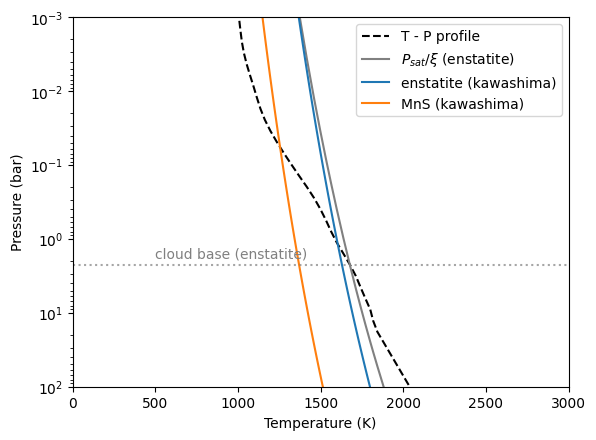
The cloud base is located at the intersection of a TP profile and the vapor saturation puressure devided by VMR.

It’s consistent with VIRGA and Kawashima-san’s private code:

plt.plot(temperature, pressure, color="black", ls="dashed", label="T - P profile")
plt.plot(temperature,
         P_enstatite / MolMR_enstatite,
         label="$P_{sat}/\\xi$ (enstatite)",
         color="gray")
parr=np.logspace(-3,2,100)
plt.plot(T_MgSiO3(parr,0.0),parr,label="enstatite (kawashima)")
plt.plot(T_MnS(parr,0.0),parr,label="MnS (kawashima)")

plt.axhline(Pbase_enstatite, color="gray", alpha=0.7, ls="dotted")
plt.text(500, Pbase_enstatite * 0.8, "cloud base (enstatite)", color="gray")

plt.yscale("log")
plt.ylim(1.e-3, 1.e2)
plt.xlim(0, 3000)
plt.gca().invert_yaxis()
plt.legend()
plt.xlabel("Temperature (K)")
plt.ylabel("Pressure (bar)")
plt.savefig("pbase.pdf", bbox_inches="tight", pad_inches=0.0)
plt.savefig("pbase.png", bbox_inches="tight", pad_inches=0.0)
plt.show()

#for key, val in all_out.items():
#    print(key)

con_mmr = all_out["condensate_mmr"]
#con_mmr
show(jpi.condensate_mmr(all_out))

Computes MMRs of clouds.

from exojax.atm.amclouds import mixing_ratio_cloud_profile
from exojax.atm.mixratio import vmr2mmr
from exojax.spec.molinfo import molmass_isotope
molmass_enstatite = molmass_isotope("MgSiO3", db_HIT=False)

MMRbase_enstatite = vmr2mmr(MolMR_enstatite, molmass_enstatite, mu)
MMRc_enstatite = mixing_ratio_cloud_profile(pressure, Pbase_enstatite, fsed, MMRbase_enstatite)

molmass_enstatite

100.3887

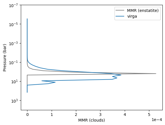
Here is the MMR distribution.

plt.figure()
plt.gca().get_xaxis().get_major_formatter().set_powerlimits([-3, 3])
plt.plot(MMRc_enstatite, pressure, color="gray", label="MMR (enstatite)")
plt.plot(con_mmr,pressure, label="virga")
plt.yscale("log")
plt.ylim(1.e-7, 10000)
plt.gca().invert_yaxis()
plt.legend()
plt.xlabel("MMR (clouds)")
plt.ylabel("Pressure (bar)")
plt.savefig("mmrcloud.pdf", bbox_inches="tight", pad_inches=0.0)
plt.savefig("mmrcloud.png", bbox_inches="tight", pad_inches=0.0)
plt.show()

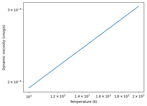
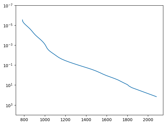
Compute dynamic viscosity in H2 atmosphere (cm/g/s)

from exojax.atm.viscosity import eta_Rosner, calc_vfactor

T = np.logspace(np.log10(1000), np.log10(2000))
vfactor, Tr = calc_vfactor("H2")
eta = eta_Rosner(T, vfactor)

plt.plot(T, eta)
plt.xscale("log")
plt.yscale("log")
plt.xlabel("Temperature (K)")
plt.ylabel("Dynamic viscosity (cm/g/s)")
plt.show()

The pressure scale height can be computed using atm.atmprof.Hatm.

from exojax.atm.atmprof import pressure_scale_height
T = 1000  #K
print("scale height=", pressure_scale_height(1.e5, T, mu), "cm")

scale height= 415722.99317937146 cm

We need a substance density of condensates.

from exojax.atm.condensate import condensate_substance_density, name2formula
deltac_enstatite = condensate_substance_density[name2formula["enstatite"]]

mu = molmass_isotope("H2")

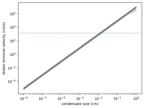
Let’s compute the terminal velocity. We can compute the terminal velocity of cloud particle using atm.vterm.vf. vmap is again applied to vf.

from exojax.atm.viscosity import calc_vfactor, eta_Rosner
from exojax.atm.vterm import terminal_velocity
from jax import vmap

vfactor, trange = calc_vfactor(atm="H2")
rarr = jnp.logspace(-6, 0, 2000)  #cm
drho = deltac_enstatite - rho
eta_fid = eta_Rosner(temperature, vfactor)

#g = 1.e5
vf_vmap = vmap(terminal_velocity, (None, None, 0, 0, 0))
vfs = vf_vmap(rarr, gravity, eta_fid, drho, rho)

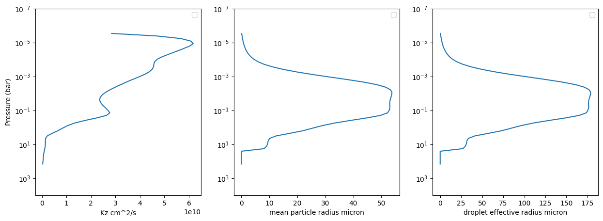
Kz_virga = all_out["kz"]
mpf = all_out["mean_particle_r"]
deff = all_out["droplet_eff_r"]

fig = plt.figure(figsize=(15,5))
ax = fig.add_subplot(131)
plt.gca().get_xaxis().get_major_formatter().set_powerlimits([-3, 3])
plt.plot(Kz_virga,pressure)
plt.yscale("log")
plt.ylim(1.e-7, 10000)
plt.gca().invert_yaxis()
plt.legend()
plt.xlabel("Kz "+str(all_out["kz_unit"]))
plt.ylabel("Pressure (bar)")


ax = fig.add_subplot(132)
plt.gca().get_xaxis().get_major_formatter().set_powerlimits([-3, 3])
plt.plot(mpf,pressure)
plt.yscale("log")
plt.ylim(1.e-7, 10000)
plt.gca().invert_yaxis()
plt.legend()
plt.xlabel("mean particle radius " +str(all_out["r_units"]))

ax = fig.add_subplot(133)
plt.gca().get_xaxis().get_major_formatter().set_powerlimits([-3, 3])
plt.plot(deff,pressure)
plt.yscale("log")
plt.ylim(1.e-7, 10000)
plt.gca().invert_yaxis()
plt.legend()
plt.xlabel("droplet effective radius " +str(all_out["r_units"]))

plt.show()

No artists with labels found to put in legend.  Note that artists whose label start with an underscore are ignored when legend() is called with no argument.
No artists with labels found to put in legend.  Note that artists whose label start with an underscore are ignored when legend() is called with no argument.
No artists with labels found to put in legend.  Note that artists whose label start with an underscore are ignored when legend() is called with no argument.

plt.plot(temperature, pressure)
plt.yscale("log")
plt.ylim(1.e-7, 10000)
plt.gca().invert_yaxis()

Kzz/L will be used to calibrate \(r_w\). following Ackerman and Marley 2001

Kzz = 3.e10  #cm2/s
sigmag = 2.0
alphav = 1.3
L = pressure_scale_height(gravity, 1500, mu)

for i in range(0, len(temperature)):
    plt.plot(rarr, vfs[i, :], alpha=0.2, color="gray")
plt.xscale("log")
plt.yscale("log")
plt.axhline(Kzz / L, label="Kzz/H", color="C2", ls="dotted")
plt.ylabel("stokes terminal velocity (cm/s)")
plt.xlabel("condensate size (cm)")

Text(0.5, 0, 'condensate size (cm)')

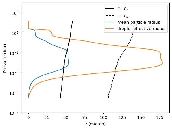
Find the intersection.

from exojax.atm.amclouds import find_rw

vfind_rw = vmap(find_rw, (None, 0, None), 0)
rw = vfind_rw(rarr, vfs, Kzz / L)

Then, \(r_g\) can be computed from \(r_w\) and other quantities.

from exojax.atm.amclouds import get_rg

rg = get_rg(rw, fsed, alphav, sigmag)

plt.plot(rg * 1.e4, pressure, label="$r=r_g$", color="black")
plt.plot(rw * 1.e4, pressure, ls="dashed", label="$r=r_w$", color="black")
plt.plot(mpf,pressure, label="mean particle radius")
plt.plot(deff,pressure, label="droplet effective radius")

plt.plot()
plt.ylim(1.e-7, 10000)
plt.xlabel("$r$ (micron)")
plt.ylabel("Pressure (bar)")
plt.yscale("log")
plt.savefig("rgrw.png")
plt.legend()

<matplotlib.legend.Legend at 0x7f6b3260a140>

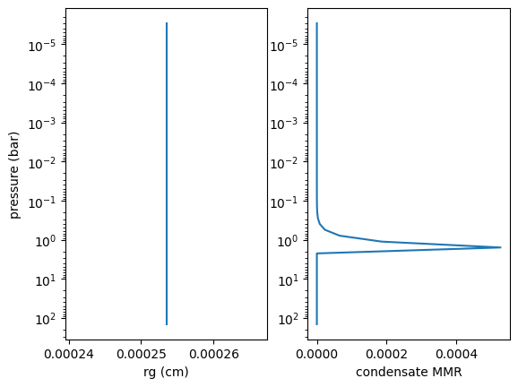
This can be simply derived using AmpAmcloud

from exojax.atm.atmphys import AmpAmcloud

amp = AmpAmcloud(pdb, bkgatm="H2")
amp.check_temperature_range(temperature)
fsed = 3.0
sigmag = 2.0
Kzz = 3.0e10

rg_layer, MMR_enstatite = amp.calc_ammodel(pressure, temperature, mu, molmass_enstatite, gravity, fsed=fsed, sigmag=sigmag, Kzz=Kzz, MMR_base=MMRbase_enstatite)


fig = plt.figure()
ax = fig.add_subplot(121)
plt.plot(rg_layer, pressure)
plt.xlabel("rg (cm)")
plt.ylabel("pressure (bar)")
plt.yscale("log")
ax.invert_yaxis()
ax = fig.add_subplot(122)
plt.plot(MMR_enstatite, pressure)
plt.xlabel("condensate MMR")
plt.yscale("log")
# plt.xscale("log")
ax.invert_yaxis()

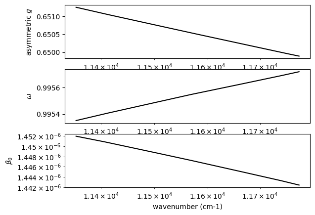
Mie Scattering

rg = np.median(rg_layer)

#mieQpar = pdb.miegrid_interpolated_values(rg, sigmag)


from exojax.utils.grids import wavenumber_grid
from exojax.spec.unitconvert import wav2nu

N = 40000
wavelength_start = 8500.0 #AA
wavelength_end = 8800.0 #AA

margin = 10  # cm-1
nus_start = wav2nu(wavelength_end, unit="AA") - margin
nus_end = wav2nu(wavelength_start, unit="AA") + margin
nugrid, wav, res = wavenumber_grid(nus_start, nus_end, N, xsmode="lpf", unit="cm-1")


from exojax.spec.opacont import OpaMie
opa = OpaMie(pdb, nugrid)
#beta0, betasct, g = opa.mieparams_vector(rg,sigmag) # if you've already generated miegrid
beta0, betasct, g = opa.mieparams_vector_direct_from_pymiescatt(rg,sigmag) # uses direct computation of Mie params using PyMieScatt

xsmode =  lpf
xsmode assumes ESLOG in wavenumber space: mode=lpf
======================================================================
The wavenumber grid should be in ascending order.
The users can specify the order of the wavelength grid by themselves.
Your wavelength grid is in *  descending  * order
======================================================================

100%|██████████| 5/5 [00:02<00:00,  1.99it/s]

fig = plt.figure()
ax = fig.add_subplot(311)
plt.plot(nugrid, g, color="black")
plt.xscale("log")
plt.ylabel("asymmetric $g$")
ax = fig.add_subplot(312)
plt.plot(nugrid, betasct/beta0, label="single scattering albedo", color="black")
plt.xscale("log")
plt.ylabel("$\\omega$")
ax = fig.add_subplot(313)
plt.plot(nugrid, beta0, label="\\beta_0", color="black")
plt.xscale("log")
plt.yscale("log")
plt.xlabel("wavenumber (cm-1)")
plt.ylabel("$\\beta_0$")

Text(0, 0.5, '$\beta_0$')

from exojax.spec.layeropacity import layer_optical_depth_clouds_lognormal
from exojax.spec.layeropacity import layer_optical_depth_cloudgeo

# set dParr by hand...
logp = jnp.log(pressure)
dlogp = 0.34755
dParr = dlogp * pressure

dtau_cloud = layer_optical_depth_clouds_lognormal(
    dParr, beta0.real, deltac_enstatite, MMR_enstatite, rg, sigmag, gravity
)

dtau_geo = layer_optical_depth_cloudgeo(
    dParr, deltac_enstatite, MMR_enstatite, rg, sigmag, gravity
)

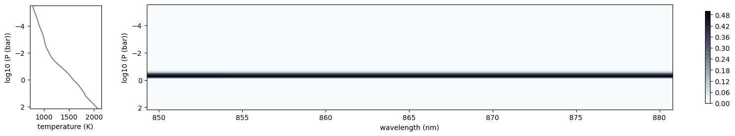
from exojax.plot.atmplot import plotcf, plottau
plotcf(nugrid, dtau_cloud, temperature, pressure, dParr, unit="nm")
plt.show()
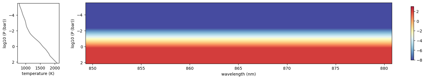
plottau(nugrid, dtau_cloud, temperature, pressure, unit="nm", vmin=-8,vmax=3)
plt.show()

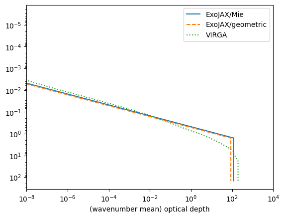
Let’s compare the optical depth profile with each other.

#virga
pressure_ = all_out['pressure']
opd_by_gas_ = all_out['opd_by_gas']


import matplotlib.pyplot as plt
fig = plt.figure()
ax = fig.add_subplot(111)
#plt.plot(np.mean(dtau_cloud,axis=1),pressure)
plt.plot(np.cumsum(np.mean(dtau_cloud,axis=1)),pressure, label="ExoJAX/Mie")
plt.plot(np.cumsum(dtau_geo),pressure,label="ExoJAX/geometric",ls="dashed")
plt.plot(opd_by_gas_,pressure_,label="VIRGA", ls="dotted")
plt.legend()
plt.xlim(1.e-8,1.e4)
ax.invert_yaxis()
plt.yscale("log")
plt.xscale("log")
plt.xlabel("(wavenumber mean) optical depth")
plt.savefig("comp_with_virga.png")