Comparison the AM geometric opacity with PieMieScatt
We import pdb with MgSiO3 to use the refractive index.
from exojax.database.pardb  import PdbCloud
miedir = "/home/kawahara/exojax/documents/tutorials/.database/particulates/virga"
#miedir = "/home/exoplanet01/exojax/documents/tutorials/.database/particulates/virga"
pdb = PdbCloud("MgSiO3", path=miedir)
/home/kawahara/exojax/documents/tutorials/.database/particulates/virga/virga.zip  exists. Remove it if you wanna re-download and unzip.
Refractive index file found:  /home/kawahara/exojax/documents/tutorials/.database/particulates/virga/MgSiO3.refrind
Miegrid file exists: /home/kawahara/exojax/documents/tutorials/.database/particulates/virga/miegrid_lognorm_MgSiO3.mg.npz
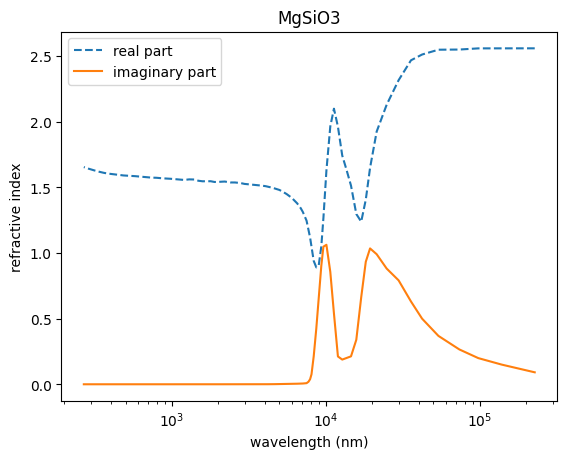
pdb has the information of refractive index in
pdb.refraction_index and pdb.refraction_index_wavelength_nm.
These values were taken from VIRGA.
Notice the refactive index has the form of \(m = n + ik\).
m = pdb.refraction_index
mwav = pdb.refraction_index_wavelength_nm

import matplotlib.pyplot as plt
plt.plot(mwav,m.real, label="real part", ls="dashed")
plt.plot(mwav,m.imag, label="imaginary part")
plt.legend()
plt.xscale("log")
plt.xlabel("wavelength (nm)")
plt.ylabel("refractive index")
plt.title("MgSiO3")
plt.savefig("mgsio3_refractive_index.png")
#plt.savefig("mgsio3_refractive_index.pdf")
plt.show()
Let’s compute the opacity of the condensate for the inicident light of 2 \(\mu\mathrm{m}\).
imie = 195
print("Incident light: " ,mwav[imie],"nm = ", mwav[imie]*1.e-3,"um")
Incident light: 268.0 nm = 0.268 um
rg_um = 0.05  # 0.1um = 100nm
sigmag = 2.0
cm2um = 1.0e4
cm2nm = 1.0e7

rg = rg_um / cm2um  # in cgs
rg_nm = rg * cm2nm

N0 = 1.0 # cm-3
from PyMieScatt import MieQ
MieQ(m[imie], mwav[imie], 2.0 * rg_nm, asDict=True)
{'Qext': 0.6246146481677305,
 'Qsca': 0.6222127380166314,
 'Qabs': 0.0024019101510991403,
 'g': 0.31392139184771023,
 'Qpr': 0.4292887594241749,
 'Qback': 0.3552936962793397,
 'Qratio': 0.5710164298658941}
PyMieScatt.Mie_Lognormal can be used to compute the extinction
coefficient [Mm-1] etc. Note that the integration range lower - upper
[nm] is very important. Be sure if the range is sufficient to cover the
main body of the lognormal distribution
from PyMieScatt import Mie_Lognormal
coeff = Mie_Lognormal(
    m[imie], mwav[imie], sigmag, 2.0 * rg_nm, N0, asDict=True, lower=1.0, upper=1000.0
)  # geoMean is a diameter in PyMieScatt
coeff
{'Bext': 0.05524251821735671,
 'Bsca': 0.05497278262294254,
 'Babs': 0.0002697355944141708,
 'bigG': 0.6015827577846368,
 'Bpr': 0.022171840043951584,
 'Bback': 0.064842639707528,
 'Bratio': 0.027327967027152126}
Do not forget the unit of Bext, Bsca, and Babs is
\(\mathrm{Mm}^{-1}\) i.e. the inverse of mega meter. To convert the
values in cgs (\(\mathrm{cm^{-1}}\)), just multiply \(10^{-8}\).
beta_ext = coeff["Bext"]*1.e-8 #Mm-1 to cm-1
Computes the optical depth for L = 10 km and \(n = 10^7 \mathrm{cm^{-3}}\)
from exojax.atm.amclouds import geometric_radius
rgeo = geometric_radius(rg, sigmag)
Assuming the large size limit (\(Q_e = 2\)), we estimate the extinction coefficient from the geometric radius.
import jax.numpy as jnp
Qe = 2 # large size limit
Qe*jnp.pi*rgeo**2
Array(4.106162e-10, dtype=float32, weak_type=True)
This is close to the extinction coefficient computed using
PyMieScatt.
beta_ext
5.524251821735671e-10