Comparing HITEMP and ExoMol
from exojax.database.core.line_strength import line_strength
from exojax.database.core.broadening  import doppler_sigma
from exojax.database.core.broadening  import gamma_hitran
from exojax.database.core.broadening  import gamma_natural
from exojax.database.core.broadening  import gamma_exomol
from exojax.database.exomol.api import MdbExomol
from exojax.database.hitemp.api import MdbHitemp
import numpy as np
import matplotlib.pyplot as plt
First of all, set a wavenumber bin in the unit of wavenumber (cm-1). Here we set the wavenumber range as \(1000 \le \nu \le 10000\) (1/cm) with the resolution of 0.01 (1/cm).
We call moldb instance with the path of par file. If the par file does not exist, moldb will try to download it from HITRAN website.
# Setting wavenumber bins and loading HITEMP database
wav = np.linspace(22930.0, 23000.0, 4000, dtype=np.float64)  # AA
nus = 1.0e8 / wav[::-1]  # cm-1
mdbCO_HITEMP = MdbHitemp(
    "CO", nus, isotope=1, gpu_transfer=True
)  # we use istope=1 for comparison
radis engine =  vaex
tosss  {'ENCRYPTION_KEY': 'Y4OG6orz1ng3xBpegpj_QmYb-3f7_OvMx6UfMiyRlTw=', 'HITRAN_USERNAME': 'gAAAAABn4pSK0S_unODzf8VGcmEv9LOE59ieBYv8sDVPZB25LRvs-c3z9_lnLlhd2gGYbMR-wOHIyQqkm-DIZ58_L2uAduTvbjJ0JBjAgZddtWgmO-TLCfI=', 'HITRAN_PASSWORD': 'gAAAAABn4pSKXNM5OmFnW_WWeFp_mPg1UlVQg2FuSPsg192eWgpSephsl1b4LuSs-QtuMupi9xUuKnmfS3V7BYudOHnYIaIZLQ==', 'HITRAN_EMAIL': 'gAAAAABn4pSK0S_unODzf8VGcmEv9LOE59ieBYv8sDVPZB25LRvs-c3z9_lnLlhd2gGYbMR-wOHIyQqkm-DIZ58_L2uAduTvbjJ0JBjAgZddtWgmO-TLCfI='}
Login successful.
Starting download from https://hitran.org/files/HITEMP/bzip2format/05_HITEMP2019.par.bz2 to 05_HITEMP2019.par.bz2
Total size to download: 14834352 bytes
05_HITEMP2019.par.bz2: 100%|██████████| 14.8M/14.8M [00:03<00:00, 3.81MB/s]
Download complete!
emf = "CO/12C-16O/Li2015"  # this is isotope=1 12C-16O
mdbCO_Li2015 =MdbExomol(emf, nus, gpu_transfer=True)
/home/kawahara/exojax/src/exojax/utils/molname.py:197: FutureWarning: e2s will be replaced to exact_molname_exomol_to_simple_molname.
  warnings.warn(
/home/kawahara/exojax/src/exojax/utils/molname.py:91: FutureWarning: exojax.utils.molname.exact_molname_exomol_to_simple_molname will be replaced to radis.api.exomolapi.exact_molname_exomol_to_simple_molname.
  warnings.warn(
/home/kawahara/exojax/src/exojax/utils/molname.py:91: FutureWarning: exojax.utils.molname.exact_molname_exomol_to_simple_molname will be replaced to radis.api.exomolapi.exact_molname_exomol_to_simple_molname.
  warnings.warn(
HITRAN exact name= (12C)(16O)
radis engine =  vaex
Total download size ['12C-16O__Li2015.def'] is: 0.000005 GB
             => Downloading from https://www.exomol.com/db/CO/12C-16O/Li2015/12C-16O__Li2015.def
Total download size ['12C-16O__Li2015.pf'] is: 0.000218 GB
             => Downloading from https://www.exomol.com/db/CO/12C-16O/Li2015/12C-16O__Li2015.pf
Total download size ['12C-16O__Li2015.states.bz2'] is: 0.000051 GB
             => Downloading from https://www.exomol.com/db/CO/12C-16O/Li2015/12C-16O__Li2015.states.bz2
/home/kawahara/anaconda3/lib/python3.10/site-packages/radis/api/exomolapi.py:1702: UserWarning: Failed to fetch size for 12C-16O__self.broad: HTTP Error 404: Not Found
  warnings.warn(f"Failed to fetch size for {pfname}: {e}", UserWarning)
/home/kawahara/anaconda3/lib/python3.10/site-packages/radis/api/exomolapi.py:1702: UserWarning: Failed to fetch size for 12C-16O__Ar.broad: HTTP Error 404: Not Found
  warnings.warn(f"Failed to fetch size for {pfname}: {e}", UserWarning)
/home/kawahara/anaconda3/lib/python3.10/site-packages/radis/api/exomolapi.py:1702: UserWarning: Failed to fetch size for 12C-16O__CH4.broad: HTTP Error 404: Not Found
  warnings.warn(f"Failed to fetch size for {pfname}: {e}", UserWarning)
/home/kawahara/anaconda3/lib/python3.10/site-packages/radis/api/exomolapi.py:1702: UserWarning: Failed to fetch size for 12C-16O__CO.broad: HTTP Error 404: Not Found
  warnings.warn(f"Failed to fetch size for {pfname}: {e}", UserWarning)
/home/kawahara/anaconda3/lib/python3.10/site-packages/radis/api/exomolapi.py:1702: UserWarning: Failed to fetch size for 12C-16O__CO2.broad: HTTP Error 404: Not Found
  warnings.warn(f"Failed to fetch size for {pfname}: {e}", UserWarning)
/home/kawahara/anaconda3/lib/python3.10/site-packages/radis/api/exomolapi.py:1702: UserWarning: Failed to fetch size for 12C-16O__H2O.broad: HTTP Error 404: Not Found
  warnings.warn(f"Failed to fetch size for {pfname}: {e}", UserWarning)
/home/kawahara/anaconda3/lib/python3.10/site-packages/radis/api/exomolapi.py:1702: UserWarning: Failed to fetch size for 12C-16O__N2.broad: HTTP Error 404: Not Found
  warnings.warn(f"Failed to fetch size for {pfname}: {e}", UserWarning)
/home/kawahara/anaconda3/lib/python3.10/site-packages/radis/api/exomolapi.py:1702: UserWarning: Failed to fetch size for 12C-16O__NH3.broad: HTTP Error 404: Not Found
  warnings.warn(f"Failed to fetch size for {pfname}: {e}", UserWarning)
/home/kawahara/anaconda3/lib/python3.10/site-packages/radis/api/exomolapi.py:1702: UserWarning: Failed to fetch size for 12C-16O__NO.broad: HTTP Error 404: Not Found
  warnings.warn(f"Failed to fetch size for {pfname}: {e}", UserWarning)
/home/kawahara/anaconda3/lib/python3.10/site-packages/radis/api/exomolapi.py:1702: UserWarning: Failed to fetch size for 12C-16O__O2.broad: HTTP Error 404: Not Found
  warnings.warn(f"Failed to fetch size for {pfname}: {e}", UserWarning)
/home/kawahara/anaconda3/lib/python3.10/site-packages/radis/api/exomolapi.py:1702: UserWarning: Failed to fetch size for 12C-16O__CS.broad: HTTP Error 404: Not Found
  warnings.warn(f"Failed to fetch size for {pfname}: {e}", UserWarning)
Total download size ['12C-16O__H2.broad', '12C-16O__He.broad', '12C-16O__air.broad', '12C-16O__self.broad', '12C-16O__Ar.broad', '12C-16O__CH4.broad', '12C-16O__CO.broad', '12C-16O__CO2.broad', '12C-16O__H2.broad', '12C-16O__H2O.broad', '12C-16O__N2.broad', '12C-16O__NH3.broad', '12C-16O__NO.broad', '12C-16O__O2.broad', '12C-16O__NH3.broad', '12C-16O__CS.broad'] is: 0.000015 GB
             => Downloading from https://www.exomol.com/db/CO/12C-16O/12C-16O__H2.broad
             => Downloading from https://www.exomol.com/db/CO/12C-16O/12C-16O__He.broad
             => Downloading from https://www.exomol.com/db/CO/12C-16O/12C-16O__air.broad
             => Downloading from https://www.exomol.com/db/CO/12C-16O/12C-16O__self.broad
Error: Couldn't download .broad file at https://www.exomol.com/db/CO/12C-16O/12C-16O__self.broad and save.
             => Downloading from https://www.exomol.com/db/CO/12C-16O/12C-16O__Ar.broad
Error: Couldn't download .broad file at https://www.exomol.com/db/CO/12C-16O/12C-16O__Ar.broad and save.
             => Downloading from https://www.exomol.com/db/CO/12C-16O/12C-16O__CH4.broad
Error: Couldn't download .broad file at https://www.exomol.com/db/CO/12C-16O/12C-16O__CH4.broad and save.
             => Downloading from https://www.exomol.com/db/CO/12C-16O/12C-16O__CO.broad
Error: Couldn't download .broad file at https://www.exomol.com/db/CO/12C-16O/12C-16O__CO.broad and save.
             => Downloading from https://www.exomol.com/db/CO/12C-16O/12C-16O__CO2.broad
Error: Couldn't download .broad file at https://www.exomol.com/db/CO/12C-16O/12C-16O__CO2.broad and save.
             => Downloading from https://www.exomol.com/db/CO/12C-16O/12C-16O__H2.broad
             => Downloading from https://www.exomol.com/db/CO/12C-16O/12C-16O__H2O.broad
Error: Couldn't download .broad file at https://www.exomol.com/db/CO/12C-16O/12C-16O__H2O.broad and save.
             => Downloading from https://www.exomol.com/db/CO/12C-16O/12C-16O__N2.broad
Error: Couldn't download .broad file at https://www.exomol.com/db/CO/12C-16O/12C-16O__N2.broad and save.
             => Downloading from https://www.exomol.com/db/CO/12C-16O/12C-16O__NH3.broad
Error: Couldn't download .broad file at https://www.exomol.com/db/CO/12C-16O/12C-16O__NH3.broad and save.
             => Downloading from https://www.exomol.com/db/CO/12C-16O/12C-16O__NO.broad
Error: Couldn't download .broad file at https://www.exomol.com/db/CO/12C-16O/12C-16O__NO.broad and save.
             => Downloading from https://www.exomol.com/db/CO/12C-16O/12C-16O__O2.broad
Error: Couldn't download .broad file at https://www.exomol.com/db/CO/12C-16O/12C-16O__O2.broad and save.
             => Downloading from https://www.exomol.com/db/CO/12C-16O/12C-16O__NH3.broad
Error: Couldn't download .broad file at https://www.exomol.com/db/CO/12C-16O/12C-16O__NH3.broad and save.
             => Downloading from https://www.exomol.com/db/CO/12C-16O/12C-16O__CS.broad
Error: Couldn't download .broad file at https://www.exomol.com/db/CO/12C-16O/12C-16O__CS.broad and save.

Summary of broadening files downloaded:
    Success: ['H2' 'He' 'air' 'H2']
    Fail: ['self' 'Ar' 'CH4' 'CO' 'CO2' 'H2O' 'N2' 'NH3' 'NO' 'O2' 'NH3' 'CS']

Note: Caching states data to the vaex format. After the second time, it will become much faster.
Molecule:  CO
Isotopologue:  12C-16O
ExoMol database:  None
Local folder:  CO/12C-16O/Li2015
Transition files:
     => File 12C-16O__Li2015.trans
Total download size ['12C-16O__Li2015.trans.bz2'] is: 0.001307 GB
             => Downloading from https://www.exomol.com/db/CO/12C-16O/Li2015/12C-16O__Li2015.trans.bz2
             => Caching the .trans.bz2 file to the vaex (.h5) format. After the second time, it will become much faster.
             => You can deleted the 'trans.bz2' file by hand.
Broadener:  H2
Broadening code level: a0
/home/kawahara/anaconda3/lib/python3.10/site-packages/radis/api/exomolapi.py:727: AccuracyWarning: The default broadening parameter (alpha = 0.07 cm^-1 and n = 0.5) are used for J'' > 80 up to J'' = 152
  warnings.warn(
Define molecular weight of CO (\(\sim 12+16=28\)), temperature (K), and pressure (bar). Also, we here assume the 100 % CO atmosphere, i.e. the partial pressure = pressure.
from exojax.database import molinfo

molecular_mass = molinfo.molmass("CO")  # molecular weight
Tfix = 1300.0  # we assume T=1300K
Pfix = 0.99  # we compute P=1 bar=0.99+0.1
Ppart = 0.01  # partial pressure of CO. here we assume a 1% CO atmosphere (very few).
partition function ratio \(q(T)\) is defined by
\(q(T) = Q(T)/Q(T_{ref})\); \(T_{ref}\)=296 K
Here, we use the partition function from HAPI
# mdbCO_HITEMP.ExomolQT(emf) #use Q(T) from Exomol/Li2015
from exojax.utils.constants import Tref_original

qt_HITEMP = mdbCO_HITEMP.qr_interp(1, Tfix, Tref_original)
qt_Li2015 = mdbCO_Li2015.qr_interp(Tfix, Tref_original)
Let us compute the line strength S(T) at temperature of Tfix.
\(S (T;s_0,\nu_0,E_l,q(T)) = S_0 \frac{Q(T_{ref})}{Q(T)} \frac{e^{- h c E_l /k_B T}}{e^{- h c E_l /k_B T_{ref}}} \frac{1- e^{- h c \nu /k_B T}}{1-e^{- h c \nu /k_B T_{ref}}}= q_r(T)^{-1} e^{ s_0 - c_2 E_l (T^{-1} - T_{ref}^{-1})} \frac{1- e^{- c_2 \nu_0/ T}}{1-e^{- c_2 \nu_0/T_{ref}}}\)
\(s_0=\log_{e} S_0\) : logsij0
\(\nu_0\): nu_lines
\(E_l\) : elower
Why the input is \(s_0 = \log_{e} S_0\) instead of \(S_0\) in SijT? This is because the direct value of \(S_0\) is quite small and we need to use float32 for jax.
Sij_HITEMP = line_strength(
    Tfix,
    mdbCO_HITEMP.logsij0,
    mdbCO_HITEMP.nu_lines,
    mdbCO_HITEMP.elower,
    qt_HITEMP,
    Tref_original,
)
Sij_Li2015 = line_strength(
    Tfix,
    mdbCO_Li2015.logsij0,
    mdbCO_Li2015.nu_lines,
    mdbCO_Li2015.elower,
    qt_Li2015,
    Tref_original,
)
Then, compute the Lorentz gamma factor (pressure+natural broadening)
\(\gamma_L = \gamma^p_L + \gamma^n_L\)
where the pressure broadning (HITEMP)
\(\gamma^p_L = (T/296K)^{-n_{air}} [ \alpha_{air} ( P - P_{part})/P_{atm} + \alpha_{self} P_{part}/P_{atm}]\)
\(P_{atm}\): 1 atm in the unit of bar (i.e. = 1.01325)
or
the pressure broadning (ExoMol)
$:raw-latex:gamma`^p_L = :raw-latex:alpha`{ref} ( T/T{ref} )^{-n_{texp}} ( P/P_{ref}), $
and the natural broadening
\(\gamma^n_L = \frac{A}{4 \pi c}\)
gammaL_HITEMP = gamma_hitran(
    Pfix,
    Tfix,
    Ppart,
    mdbCO_HITEMP.n_air,
    mdbCO_HITEMP.gamma_air,
    mdbCO_HITEMP.gamma_self,
) + gamma_natural(mdbCO_HITEMP.A)

gammaL_Li2015 = gamma_exomol(
    Pfix, Tfix, mdbCO_Li2015.n_Texp, mdbCO_Li2015.alpha_ref
) + gamma_natural(mdbCO_Li2015.A)
Thermal broadening
\(\sigma_D^{t} = \sqrt{\frac{k_B T}{M m_u}} \frac{\nu_0}{c}\)
# thermal doppler sigma
sigmaD_HITEMP = doppler_sigma(mdbCO_HITEMP.nu_lines, Tfix, molecular_mass)
sigmaD_Li2015 = doppler_sigma(mdbCO_Li2015.nu_lines, Tfix, molecular_mass)
Then, the line center…
In HITRAN database, a slight pressure shift can be included using \(\delta_{air}\): \(\nu_0(P) = \nu_0 + \delta_{air} P\). But this shift is quite a bit.
# line center
nu0_HITEMP = mdbCO_HITEMP.nu_lines
nu0_Li2015 = mdbCO_Li2015.nu_lines
We use Direct LFP.
from exojax.opacity.initspec import init_lpf
from exojax.opacity.lpf.lpf import xsvector

numatrix_HITEMP = init_lpf(mdbCO_HITEMP.nu_lines, nus)
xsv_HITEMP = xsvector(numatrix_HITEMP, sigmaD_HITEMP, gammaL_HITEMP, Sij_HITEMP)

numatrix_Li2015 = init_lpf(mdbCO_Li2015.nu_lines, nus)
xsv_Li2015 = xsvector(numatrix_Li2015, sigmaD_Li2015, gammaL_Li2015, Sij_Li2015)
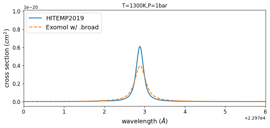
fig = plt.figure(figsize=(10, 4))
ax = fig.add_subplot(111)
plt.plot(wav[::-1], xsv_HITEMP, lw=2, label="HITEMP2019")
plt.plot(wav[::-1], xsv_Li2015, lw=2, ls="dashed", label="Exomol w/ .broad")
plt.xlim(22970, 22976)
plt.xlabel("wavelength ($\AA$)", fontsize=14)
plt.ylabel("cross section ($cm^{2}$)", fontsize=14)
plt.legend(loc="upper left", fontsize=14)
plt.tick_params(labelsize=12)
plt.savefig("co_comparison.pdf", bbox_inches="tight", pad_inches=0.0)
plt.savefig("co_comparison.png", bbox_inches="tight", pad_inches=0.0)
plt.title("T=1300K,P=1bar")
plt.show()