Ackerman and Marley Cloud Model

Here, we try to compute a cloud opacity using Ackerman and Marley Model. Although atmphys.AmpAmcloud can easily compute the parameters of the AM model, we here try to run the methods one by one. We consider enstatite (MgSiO3) and Fe clouds.

import jax.numpy as jnp
import matplotlib.pyplot as plt
import numpy as np

Sets a simple atmopheric model. We need the density of atmosphere.

from exojax.utils.constants import kB, m_u
from exojax.atm.atmprof import pressure_layer_logspace
from exojax.utils.astrofunc import gravity_jupiter

Parr, dParr, k = pressure_layer_logspace(log_pressure_top=-4., log_pressure_btm=6.0, nlayer=100)
alpha = 0.097
T0 = 1200.
Tarr = T0 * (Parr)**alpha

mu = 2.3  # mean molecular weight
R = kB / (mu * m_u)
rho = Parr / (R * Tarr)

gravity = gravity_jupiter(1.0, 1.0)

The solar abundance can be obtained using utils.zsol.nsol. Here, we assume a maximum mol Mixing Ratio for MgSiO3 and Fe from solar abundance.

from exojax.utils.zsol import nsol

n = nsol()  #solar abundance
MolMR_enstatite = np.min([n["Mg"], n["Si"], n["O"] / 3])
MolMR_Fe = n["Fe"]

Vapor saturation pressures can be obtained using atm.psat

from exojax.atm.psat import psat_enstatite_AM01, psat_Fe_AM01, _psat_Fe_solid

P_enstatite = psat_enstatite_AM01(Tarr)
P_fe_sol = psat_Fe_AM01(Tarr)
#P_fe_sol = _psat_Fe_solid(Tarr) #considers only solid Fe

Computes a cloud base pressure.

from exojax.atm.amclouds import compute_cloud_base_pressure

Pbase_enstatite = compute_cloud_base_pressure(Parr, P_enstatite, MolMR_enstatite)
Pbase_Fe_sol = compute_cloud_base_pressure(Parr, P_fe_sol, MolMR_Fe)

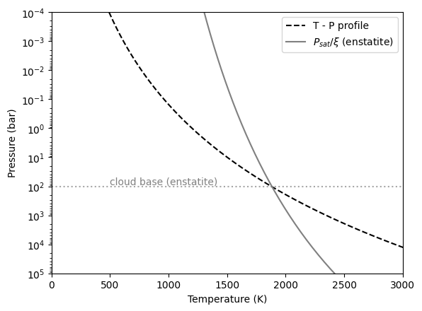
The cloud base is located at the intersection of a TP profile and the vapor saturation puressure devided by VMR.

plt.plot(Tarr, Parr, color="black", ls="dashed", label="T - P profile")
plt.plot(Tarr,
         P_enstatite / MolMR_enstatite,
         label="$P_{sat}/\\xi$ (enstatite)",
         color="gray")
plt.axhline(Pbase_enstatite, color="gray", alpha=0.7, ls="dotted")
plt.text(500, Pbase_enstatite * 0.8, "cloud base (enstatite)", color="gray")

plt.plot(Tarr, P_fe_sol / MolMR_Fe, label="$P_{sat}/\\xi$ (Fe)", color="black")
plt.axhline(Pbase_Fe_sol, color="black", alpha=0.7, ls="dotted")
plt.text(500, Pbase_Fe_sol * 0.8, "cloud base (Fe)", color="black")

plt.yscale("log")
plt.ylim(1.e-4, 1.e5)
plt.xlim(0, 3000)
plt.gca().invert_yaxis()
plt.legend()
plt.xlabel("Temperature (K)")
plt.ylabel("Pressure (bar)")
plt.savefig("pbase.pdf", bbox_inches="tight", pad_inches=0.0)
plt.savefig("pbase.png", bbox_inches="tight", pad_inches=0.0)
plt.show()

Compute Mass Mixing Ratio (MMRs) of clouds. In this block, we first convert mol mixing ratio of condensates to MMR, then computes a cloud profile.

from exojax.atm.amclouds import mixing_ratio_cloud_profile
from exojax.spec.molinfo import molmass_isotope
from exojax.atm.mixratio import vmr2mmr
fsed = 3.
muc_enstatite = molmass_isotope("MgSiO3")
MMRbase_enstatite = vmr2mmr(MolMR_enstatite, muc_enstatite,mu)
MMRc_enstatite = mixing_ratio_cloud_profile(Parr, Pbase_enstatite, fsed, MMRbase_enstatite)

muc_Fe = molmass_isotope("Fe")
MMRbase_Fe = vmr2mmr(MolMR_Fe,muc_Fe,mu)
MMRc_Fe = mixing_ratio_cloud_profile(Parr, Pbase_Fe_sol, fsed, MMRbase_Fe)

['H2O', 'CO2', 'O3', 'N2O', 'CO', 'CH4', 'O2', 'NO', 'SO2', 'NO2', 'NH3', 'HNO3', 'OH', 'HF', 'HCl', 'HBr', 'HI', 'ClO', 'OCS', 'H2CO', 'HOCl', 'N2', 'HCN', 'CH3Cl', 'H2O2', 'C2H2', 'C2H6', 'PH3', 'COF2', 'SF6', 'H2S', 'HCOOH', 'HO2', 'O', 'ClONO2', 'NO+', 'HOBr', 'C2H4', 'CH3OH', 'CH3Br', 'CH3CN', 'CF4', 'C4H2', 'HC3N', 'H2', 'CS', 'SO3', 'C2N2', 'COCl2', 'SO', 'CH3F', 'GeH4', 'CS2', 'CH3I', 'NF3']
['H2O', 'CO2', 'O3', 'N2O', 'CO', 'CH4', 'O2', 'NO', 'SO2', 'NO2', 'NH3', 'HNO3', 'OH', 'HF', 'HCl', 'HBr', 'HI', 'ClO', 'OCS', 'H2CO', 'HOCl', 'N2', 'HCN', 'CH3Cl', 'H2O2', 'C2H2', 'C2H6', 'PH3', 'COF2', 'SF6', 'H2S', 'HCOOH', 'HO2', 'O', 'ClONO2', 'NO+', 'HOBr', 'C2H4', 'CH3OH', 'CH3Br', 'CH3CN', 'CF4', 'C4H2', 'HC3N', 'H2', 'CS', 'SO3', 'C2N2', 'COCl2', 'SO', 'CH3F', 'GeH4', 'CS2', 'CH3I', 'NF3']

/home/kawahara/exojax/src/exojax/spec/molinfo.py:64: UserWarning: db_HIT is set as True, but the molecular name 'MgSiO3' does not exist in the HITRAN database. So set db_HIT as False. For reference, all the available molecules in the HITRAN database are as follows:
  warnings.warn(warn_msg, UserWarning)
/home/kawahara/exojax/src/exojax/spec/molinfo.py:64: UserWarning: db_HIT is set as True, but the molecular name 'Fe' does not exist in the HITRAN database. So set db_HIT as False. For reference, all the available molecules in the HITRAN database are as follows:
  warnings.warn(warn_msg, UserWarning)

The followings are the base pressures for enstatite and Fe.

print(Pbase_enstatite, Pbase_Fe_sol)

114.975746 77426.445

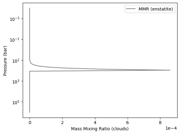
Here is the MMR distribution.

plt.figure()
plt.gca().get_xaxis().get_major_formatter().set_powerlimits([-3, 3])
plt.plot(MMRc_enstatite, Parr, color="gray", label="MMR (enstatite)")
plt.plot(MMRc_Fe, Parr, color="black", ls="dashed", label="MMR (Fe)")



plt.yscale("log")
#plt.ylim(1.e-7, 10000)
plt.gca().invert_yaxis()
plt.legend()
plt.xlabel("Mass Mixing Ratio (clouds)")
plt.ylabel("Pressure (bar)")
plt.savefig("mmrcloud.pdf", bbox_inches="tight", pad_inches=0.0)
plt.savefig("mmrcloud.png", bbox_inches="tight", pad_inches=0.0)
plt.show()

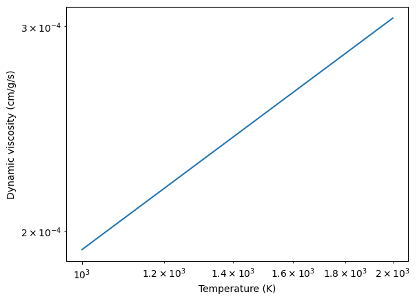
Computes dynamic viscosity in H2 atmosphere (cm/g/s)

from exojax.atm.viscosity import eta_Rosner, calc_vfactor

T = np.logspace(np.log10(1000), np.log10(2000))
vfactor, Tr = calc_vfactor("H2")
eta = eta_Rosner(T, vfactor)

plt.plot(T, eta)
plt.xscale("log")
plt.yscale("log")
plt.xlabel("Temperature (K)")
plt.ylabel("Dynamic viscosity (cm/g/s)")
plt.show()

The pressure scale height can be computed using atm.atmprof.Hatm.

from exojax.atm.atmprof import pressure_scale_height
T = 1000  #K
print("scale height=", pressure_scale_height(1.e5, T, mu), "cm")

scale height= 361498.2549385839 cm

We need the substance density of condensates.

from exojax.atm.condensate import condensate_substance_density, name2formula

deltac_enstatite = condensate_substance_density[name2formula["enstatite"]]
deltac_Fe = condensate_substance_density["Fe"]

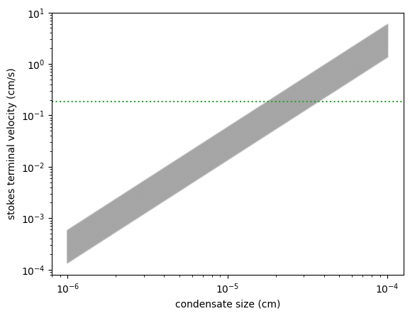
Let’s compute the terminal velocity. We can compute the terminal velocity of cloud particle using atm.vterm.vf. vmap is again applied to vf.

from exojax.atm.viscosity import calc_vfactor, eta_Rosner
from exojax.atm.vterm import terminal_velocity
from jax import vmap

vfactor, trange = calc_vfactor(atm="H2")
rarr = jnp.logspace(-6, -4, 2000)  #cm
drho = deltac_enstatite - rho
eta_fid = eta_Rosner(Tarr, vfactor)

g = 1.e5
vf_vmap = vmap(terminal_velocity, (None, None, 0, 0, 0))
vfs = vf_vmap(rarr, g, eta_fid, drho, rho)

Kzz/L will be used to calibrate \(r_w\). following Ackerman and Marley 2001

#sigmag:sigmag parameter (geometric standard deviation) in the lognormal distribution of condensate size, defined by (9) in AM01, must be sigmag > 1

Kzz = 1.e5  #cm2/s
sigmag = 2.0 # > 1
alphav = 1.3
L = pressure_scale_height(g, 1500, mu)

Kzz/L

0.18441767216274083

for i in range(0, len(Tarr)):
    plt.plot(rarr, vfs[i, :], alpha=0.2, color="gray")
plt.xscale("log")
plt.yscale("log")
plt.axhline(Kzz / L, label="Kzz/H", color="C2", ls="dotted")
plt.ylabel("stokes terminal velocity (cm/s)")
plt.xlabel("condensate size (cm)")

Text(0.5, 0, 'condensate size (cm)')

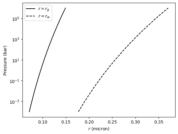
Find the intersection.

from exojax.atm.amclouds import find_rw

vfind_rw = vmap(find_rw, (None, 0, None), 0)
rw = vfind_rw(rarr, vfs, Kzz / L)

Then, \(r_g\) can be computed from \(r_w\) and other quantities.

from exojax.atm.amclouds import get_rg

rg = get_rg(rw, fsed, alphav, sigmag)

plt.plot(rg * 1.e4, Parr, label="$r=r_g$", color="black")
plt.plot(rw * 1.e4, Parr, ls="dashed", label="$r=r_w$", color="black")
#plt.ylim(1.e-7, 10000)
plt.xlabel("$r$ (micron)")
plt.ylabel("Pressure (bar)")
plt.yscale("log")
plt.savefig("rgrw.png")
plt.legend()

<matplotlib.legend.Legend at 0x7f7fac15aad0>

These processes can be reprodced using AmpAmcloud, which uses PdbCloud as one of the input arguments. Here, we show an example:

from exojax.atm.atmphys import AmpAmcloud
from exojax.spec.pardb import PdbCloud
pdb_enstatite = PdbCloud("MgSiO3")
pdb_Fe = PdbCloud("Fe")

amp = AmpAmcloud(pdb_enstatite,bkgatm="H2")
rg, MMRc = amp.calc_ammodel(Parr,Tarr,mu,MMRc_enstatite,gravity,fsed,sigmag,Kzz,MMRbase_enstatite,alphav=alphav)

.database/particulates/virga/virga.zip  exists. Remove it if you wanna re-download and unzip.
Refractive index file found:  .database/particulates/virga/MgSiO3.refrind
Miegrid file does not exist at  .database/particulates/virga/miegrid_lognorm_MgSiO3.mg.npz
Generate miegrid file using pdb.generate_miegrid if you use Mie scattering
.database/particulates/virga/virga.zip  exists. Remove it if you wanna re-download and unzip.
Refractive index file found:  .database/particulates/virga/Fe.refrind
Miegrid file does not exist at  .database/particulates/virga/miegrid_lognorm_Fe.mg.npz
Generate miegrid file using pdb.generate_miegrid if you use Mie scattering

We found here the particle size is basically sub-micron.

Here, we try to use the geometric cross section instead though this is sometimes wrong, depending on the wavelength.

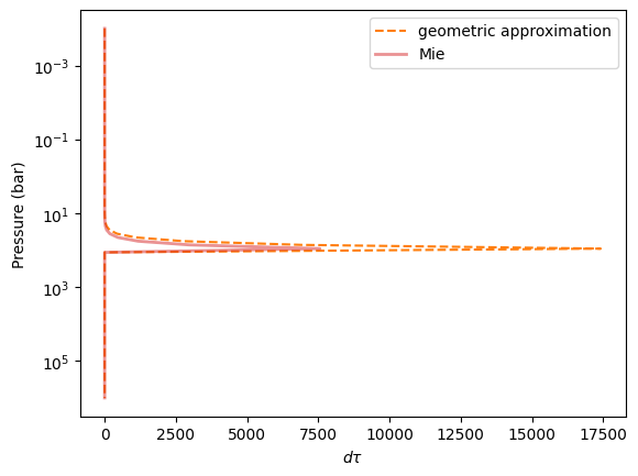
from exojax.spec.layeropacity import layer_optical_depth_cloudgeo

dtau_enstatite = layer_optical_depth_cloudgeo(Parr, deltac_enstatite, MMRc_enstatite, rg, sigmag, g)
dtau_Fe = layer_optical_depth_cloudgeo(Parr, deltac_Fe, MMRc_Fe, rg, sigmag, g)

/home/kawahara/exojax/src/exojax/spec/dtau_mmwl.py:14: FutureWarning: dtau_mmwl might be removed in future.
  warnings.warn("dtau_mmwl might be removed in future.", FutureWarning)

The Mie scattering can be computed using OpaMie.

from exojax.utils.grids import wavenumber_grid
from exojax.spec.unitconvert import wav2nu

N = 1000
wavelength_start = 5000.0 #AA
wavelength_end = 15000.0 #AA


margin = 10  # cm-1
nus_start = wav2nu(wavelength_end, unit="AA") - margin
nus_end = wav2nu(wavelength_start, unit="AA") + margin
nugrid, wav, res = wavenumber_grid(nus_start, nus_end, N, xsmode="lpf", unit="cm-1")



from exojax.spec.opacont import OpaMie
opa_enstatite = OpaMie(pdb_enstatite, nugrid)
opa_Fe = OpaMie(pdb_Fe, nugrid)

rg=1.e-4 #0.1um
#beta0, betasct, g = opa.mieparams_vector(rg,sigmag) # if you've already generated miegrid
beta0, betasct, g = opa_enstatite.mieparams_vector_direct_from_pymiescatt(rg,sigmag) # uses direct computation of Mie params using PyMieScatt
beta0_Fe, betasct_Fe, g_Fe = opa_Fe.mieparams_vector_direct_from_pymiescatt(rg,sigmag) # uses direct computation of Mie params using PyMieScatt


from exojax.spec.layeropacity import layer_optical_depth_clouds_lognormal

dtau_enstatite_mie = layer_optical_depth_clouds_lognormal(
    dParr, beta0, deltac_enstatite, MMRc_enstatite, rg, sigmag, gravity
)
dtau_Fe_mie = layer_optical_depth_clouds_lognormal(
    dParr, beta0_Fe, deltac_Fe, MMRc_Fe, rg, sigmag, gravity
)

/home/kawahara/exojax/src/exojax/utils/grids.py:142: UserWarning: Resolution may be too small. R=907.6757560767178
  warnings.warn('Resolution may be too small. R=' + str(resolution),

xsmode =  lpf
xsmode assumes ESLOG in wavenumber space: mode=lpf
======================================================================
The wavenumber grid should be in ascending order.
The users can specify the order of the wavelength grid by themselves.
Your wavelength grid is in *  descending  * order
======================================================================

100%|██████████| 63/63 [00:17<00:00,  3.55it/s]
100%|██████████| 63/63 [00:20<00:00,  3.09it/s]

The difference of the geometric approximation and Mie scattering is a bit.

fig = plt.figure()
ax=fig.add_subplot(121)
plt.plot(dtau_enstatite, Parr, color="C1", ls="dashed", label="geometric approximation")
plt.plot(np.median(dtau_enstatite_mie,axis=1), Parr, color="C3", label="Mie",alpha=0.5,lw=2)
plt.legend()
plt.yscale("log")
plt.xlabel("$d\\tau$")
plt.ylabel("Pressure (bar)")
#plt.xscale("log")
plt.gca().invert_yaxis()

ax=fig.add_subplot(122)
plt.plot(dtau_Fe, Parr, color="C2", ls="dashed", label="geometric approximation")
plt.plot(np.median(dtau_Fe_mie,axis=1), Parr, color="C4",alpha=0.5, label="Mie",lw=2)

plt.legend()
plt.yscale("log")
plt.xlabel("$d\\tau$")
#plt.xscale("log")
plt.gca().invert_yaxis()
plt.show()

Let’s compare with CIA

#CIA

from exojax.spec import contdb
cdbH2H2 = contdb.CdbCIA('.database/H2-H2_2011.cia', nugrid)

H2-H2

from exojax.spec.layeropacity import layer_optical_depth_CIA
from exojax.atm.mixratio import mmr2vmr

mmrH2 = 0.74
molmassH2 = molmass_isotope("H2")
vmrH2 = mmr2vmr(mmrH2, mu, molmassH2)
dtaucH2H2 = layer_optical_depth_CIA(
    nugrid,
    Tarr,
    Parr,
    dParr,
    vmrH2,
    vmrH2,
    mu,
    gravity,
    cdbH2H2.nucia,
    cdbH2H2.tcia,
    cdbH2H2.logac,
)

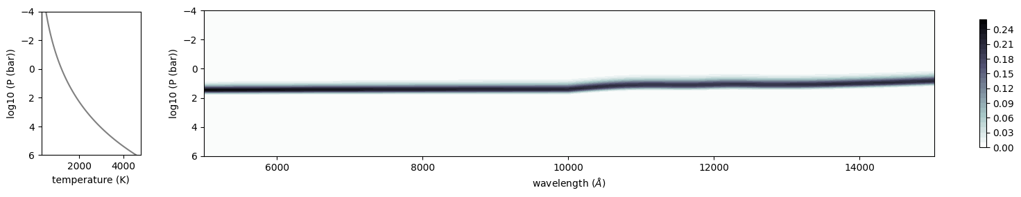
dtau = dtaucH2H2 + dtau_enstatite_mie+ dtau_Fe_mie

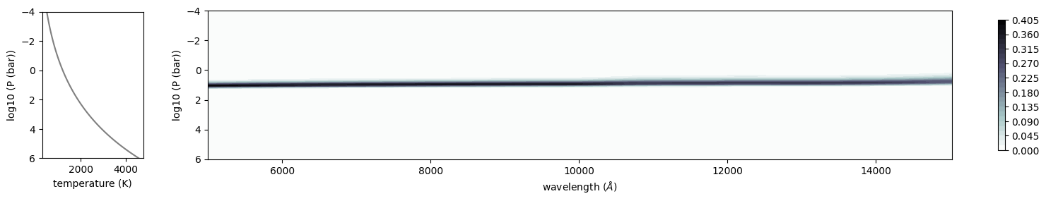
from exojax.plot.atmplot import plotcf

plotcf(nugrid, dtau, Tarr, Parr, dParr, unit="AA")
plt.show()

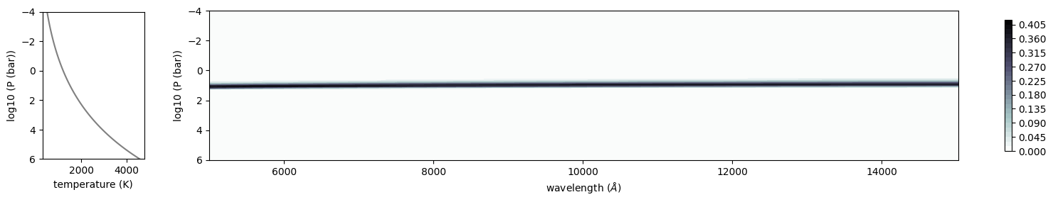
from exojax.plot.atmplot import plotcf

plotcf(nugrid, dtaucH2H2, Tarr, Parr, dParr, unit="AA")
plt.show()

from exojax.plot.atmplot import plotcf

plotcf(nugrid,
       dtau_enstatite_mie,
       Tarr,
       Parr,
       dParr,
       unit="AA")
plt.show()

from exojax.spec import planck
from exojax.spec.rtransfer import rtrun_emis_pureabs_fbased2st as rtrun
#from exojax.spec.rtransfer import rtrun_emis_pureabs_ibased as rtrun
sourcef = planck.piBarr(Tarr, nugrid)
F0 = rtrun(dtau, sourcef)
F0CIA = rtrun(dtaucH2H2, sourcef)
F0cl = rtrun(dtau_enstatite[:, None] + np.zeros_like(dtaucH2H2), sourcef)

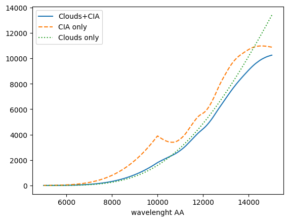
In this case, the effect of clouds and CIA are comparable with each other

plt.plot(wav, F0, label="Clouds+CIA")
plt.plot(wav, F0CIA, label="CIA only", ls="dashed")
plt.plot(wav, F0cl, label="Clouds only", ls="dotted")
plt.xlabel("wavelenght AA")
plt.legend()
plt.show()