Forward Modelling of a Many Lines Spectrum using DIT
Here, we try to compute a emission spectrum using DIT.
from exojax.spec import rtransfer as rt
from exojax.spec import dit
from exojax.spec import lpf
import numpy as np
import matplotlib.pyplot as plt
plt.style.use('bmh')
#ATMOSPHERE
NP=100
T0=1295.0 #K
Parr, dParr, k=rt.pressure_layer(NP=NP)
Tarr = T0*(Parr)**0.1
We set a wavenumber grid using wavenumber_grid. Specify xsmode=“dit” though it is not mandatory. DIT uses FFT, so the (internal) wavenumber grid should be linear. But, you can also use a nonlinear grid. In this case, the interpolation (jnp.interp) is used.
from exojax.utils.grids import wavenumber_grid
nus,wav,res=wavenumber_grid(22900,23000,10000,unit="AA",xsmode="dit")
nugrid is linear: mode= dit
Loading a molecular database of CO and CIA (H2-H2)…
from exojax.spec import api, contdb
mdbCO=api.MdbExomol('.database/CO/12C-16O/Li2015',nus)
cdbH2H2=contdb.CdbCIA('.database/H2-H2_2011.cia',nus)
Background atmosphere:  H2
Reading transition file
.broad is used.
Broadening code level= a0
default broadening parameters are used for  71  J lower states in  152  states
H2-H2
from exojax.spec import molinfo
molmassCO=molinfo.molmass("CO")
Computing the relative partition function,
from jax import vmap
qt=vmap(mdbCO.qr_interp)(Tarr)
Pressure and Natural broadenings
from jax import jit
from exojax.spec.exomol import gamma_exomol
from exojax.spec import gamma_natural

gammaLMP = jit(vmap(gamma_exomol,(0,0,None,None)))\
        (Parr,Tarr,mdbCO.n_Texp,mdbCO.alpha_ref)
gammaLMN=gamma_natural(mdbCO.A)
gammaLM=gammaLMP+gammaLMN[None,:]
Doppler broadening
from exojax.spec import doppler_sigma
sigmaDM=jit(vmap(doppler_sigma,(None,0,None)))\
        (mdbCO.nu_lines,Tarr,molmassCO)
And line strength
from exojax.spec import SijT
SijM=jit(vmap(SijT,(0,None,None,None,0)))\
    (Tarr,mdbCO.logsij0,mdbCO.nu_lines,mdbCO.elower,qt)
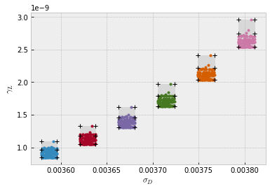
DIT requires the grids of sigmaD, gammaL, and wavenumber. For the emission spectrum, this grids should be prepared for each layer. dit.dgmatrix can compute these grids.
dgm_sigmaD=dit.dgmatrix(sigmaDM)
dgm_gammaL=dit.dgmatrix(gammaLM)

#you can change the resolution
#dgm_sigmaD=dit.dgmatrix(sigmaDM,res=0.1)
#dgm_gammaL=dit.dgmatrix(gammaLM,res=0.1)
We can check how the grids are set for each layers using plot.ditplot.plot_dgm
#show the DIT grids
from exojax.plot.ditplot import plot_dgm
plot_dgm(dgm_sigmaD,dgm_gammaL,sigmaDM,gammaLM,0,6)
from exojax.spec import initspec
cnu,indexnu,pmarray=initspec.init_dit(mdbCO.nu_lines,nus)
Let’s compute a cross section matrix.
xsmdit=dit.xsmatrix(cnu,indexnu,pmarray,sigmaDM,gammaLM,SijM,nus,dgm_sigmaD,dgm_gammaL)
Some elements may be small negative values because of error for DIT. you can just use jnp.abs
import jax.numpy as jnp
print(len(xsmdit[xsmdit<0.0]),"/",len((xsmdit).flatten()))
print("min value=",jnp.min(xsmdit[xsmdit<0.0]))
148782 / 1000000
min value= -3.1114657e-28
xsmdit=jnp.abs(xsmdit)
We also compute the cross section using the direct computation (LPF) for the comparison purpose.
#direct LPF for comparison
from exojax.spec.lpf import xsmatrix
numatrix=initspec.init_lpf(mdbCO.nu_lines,nus)
xsmdirect=xsmatrix(numatrix,sigmaDM,gammaLM,SijM)
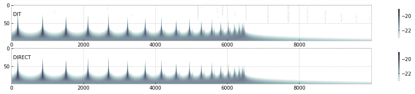
Let’s see the cross section matrix!
import numpy as np
import matplotlib.pyplot as plt
fig=plt.figure(figsize=(20,3))
ax=fig.add_subplot(211)
c=plt.imshow(np.log10(xsmdit),cmap="bone_r",vmin=-23,vmax=-19)
plt.colorbar(c,shrink=0.8)
plt.text(50,30,"DIT")
ax.set_aspect(0.1/ax.get_data_ratio())
ax.set_aspect(0.1/ax.get_data_ratio())
ax=fig.add_subplot(212)
c=plt.imshow(np.log10(xsmdirect),cmap="bone_r",vmin=-23,vmax=-19)
plt.colorbar(c,shrink=0.8)
plt.text(50,30,"DIRECT")
ax.set_aspect(0.1/ax.get_data_ratio())
plt.show()
/tmp/ipykernel_27849/1125883551.py:5: RuntimeWarning: divide by zero encountered in log10
  c=plt.imshow(np.log10(xsmdit),cmap="bone_r",vmin=-23,vmax=-19)
computing delta tau for CO
from exojax.spec.rtransfer import dtauM
Rp=0.88
Mp=33.2
g=2478.57730044555*Mp/Rp**2
#g=1.e5 #gravity cm/s2
MMR=0.0059 #mass mixing ratio
dtaum=dtauM(dParr,xsmdit,MMR*np.ones_like(Tarr),molmassCO,g)
dtaumdirect=dtauM(dParr,xsmdirect,MMR*np.ones_like(Tarr),molmassCO,g)
computing delta tau for CIA
from exojax.spec.rtransfer import dtauCIA
mmw=2.33 #mean molecular weight
mmrH2=0.74
molmassH2=molinfo.molmass("H2")
vmrH2=(mmrH2*mmw/molmassH2) #VMR
dtaucH2H2=dtauCIA(nus,Tarr,Parr,dParr,vmrH2,vmrH2,\
            mmw,g,cdbH2H2.nucia,cdbH2H2.tcia,cdbH2H2.logac)
The total delta tau is a summation of them
dtau=dtaum+dtaucH2H2
dtaudirect=dtaumdirect+dtaucH2H2
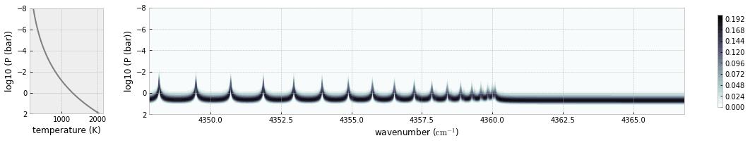
you can plot a contribution function using exojax.plot.atmplot
from exojax.plot.atmplot import plotcf
plotcf(nus,dtau,Tarr,Parr,dParr)
plt.show()
radiative transfering…
from exojax.spec import planck
from exojax.spec.rtransfer import rtrun
sourcef = planck.piBarr(Tarr,nus)
F0=rtrun(dtau,sourcef)
F0direct=rtrun(dtaudirect,sourcef)
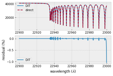
The difference is very small except around the edge (even for this it’s only 1%).
fig=plt.figure()
ax=fig.add_subplot(211)
plt.plot(wav[::-1],F0,label="DIT")
plt.plot(wav[::-1],F0direct,ls="dashed",label="direct")
plt.legend()
ax=fig.add_subplot(212)
plt.plot(wav[::-1],(F0-F0direct)/np.median(F0direct)*100,label="DIT")
plt.legend()
plt.ylabel("residual (%)")
plt.xlabel("wavelength ($\AA$)")
plt.show()
To apply response, we need to convert the wavenumber grid from ESLIN to ESLOG.
import jax.numpy as jnp
nuslog=np.logspace(np.log10(nus[0]),np.log10(nus[-1]),len(nus))
F0log=jnp.interp(nuslog,nus,F0)
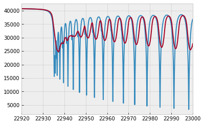
applying an instrumental response and planet/stellar rotation to the raw spectrum
from exojax.spec import response
from exojax.utils.constants import c
import jax.numpy as jnp

wavd=jnp.linspace(22920,23000,500) #observational wavelength grid
nusd = 1.e8/wavd[::-1]

RV=10.0 #RV km/s
vsini=20.0 #Vsini km/s
u1=0.0 #limb darkening u1
u2=0.0 #limb darkening u2

R=100000.
beta=c/(2.0*np.sqrt(2.0*np.log(2.0))*R) #IP sigma need check

Frot=response.rigidrot(nuslog,F0log,vsini,u1,u2)
F=response.ipgauss_sampling(nusd,nuslog,Frot,beta,RV)
plt.plot(wav[::-1],F0)
plt.plot(wavd[::-1],F)
plt.xlim(22920,23000)
(22920.0, 23000.0)