HMC-NUTS Retrieval of a Methane High-Resolution Emission Spectrum
last update: September 7th (2024) Hajime Kawahara ExoJAX v1.6
In this tutorial, we try to fit the ExoJAX emission model to a mock high-resolution spectrum. This spectrum was computed assuming a powerlaw temperature profile and CH4 opacity + CIA.
In this tutorial, we use PreMODIT as an opacity calculator.
""" Reverse modeling of Methane emission spectrum using MODIT
"""
# coding: utf-8
import numpy as np
import matplotlib.pyplot as plt
from jax import random
import jax.numpy as jnp
import pandas as pd
import pkg_resources
from exojax.rt import ArtEmisPure
from exojax.database.exomol.api import MdbExomol
from exojax.opacity import OpaPremodit
from exojax.database.contdb  import CdbCIA
from exojax.opacity import OpaCIA
from exojax.postproc.response import ipgauss_sampling
from exojax.postproc.spin_rotation import convolve_rigid_rotation
from exojax.database import molinfo
from exojax.utils.grids import nu2wav
from exojax.utils.grids import wavenumber_grid
from exojax.utils.grids import velocity_grid
from exojax.utils.astrofunc import gravity_jupiter
from exojax.utils.instfunc import resolution_to_gaussian_std
from exojax.test.data import SAMPLE_SPECTRA_CH4_NEW
/home/kawahara/exojax/src/exojax/spec/dtau_mmwl.py:14: FutureWarning: dtau_mmwl might be removed in future.
  warnings.warn("dtau_mmwl might be removed in future.", FutureWarning)
# if you wanna use FP64
#from jax import config
#config.update("jax_enable_x64", True)
We use numpyro as a probabilistic programming language (PPL). We have other options such as BlackJAX, PyMC etc.
# PPL
import arviz
from numpyro.diagnostics import hpdi
from numpyro.infer import Predictive
from numpyro.infer import MCMC, NUTS
import numpyro
import numpyro.distributions as dist
We use a sample data of the methane emission spectrum in ExoJAX, normlized it, and add Gaussian noise.
# loading the data
filename = pkg_resources.resource_filename(
    'exojax', 'data/testdata/' + SAMPLE_SPECTRA_CH4_NEW)
dat = pd.read_csv(filename, delimiter=",", names=("wavenumber", "flux"))
nusd = dat['wavenumber'].values
flux = dat['flux'].values
wavd = nu2wav(nusd, wavelength_order="ascending")
/home/kawahara/exojax/src/exojax/utils.grids.py:62: UserWarning: Both input wavelength and output wavenumber are in ascending order.
  warnings.warn(
sigmain = 0.05
norm = 20000
np.random.seed(1)
nflux = flux / norm + np.random.normal(0, sigmain, len(wavd))
We first set the wavenumber grid enough to cover the observed spectrum.
Nx = 7500
nu_grid, wav, res = wavenumber_grid(np.min(wavd) - 10.0,
                                    np.max(wavd) + 10.0,
                                    Nx,
                                    unit='AA',
                                    xsmode='premodit', wavelength_order="ascending")
xsmode =  premodit
xsmode assumes ESLOG in wavenumber space: xsmode=premodit
======================================================================
The wavenumber grid should be in ascending order.
The users can specify the order of the wavelength grid by themselves.
Your wavelength grid is in *  ascending  * order
======================================================================
/home/kawahara/exojax/src/exojax/utils.grids.py:62: UserWarning: Both input wavelength and output wavenumber are in ascending order.
  warnings.warn(
/home/kawahara/exojax/src/exojax/utils.grids.py:62: UserWarning: Both input wavelength and output wavenumber are in ascending order.
  warnings.warn(
/home/kawahara/exojax/src/exojax/utils/grids.py:144: UserWarning: Resolution may be too small. R=617160.1067701889
  warnings.warn("Resolution may be too small. R=" + str(resolution), UserWarning)
We would analyze the emission spectrum. So, we use ArtEmisPure as
art (Atmospheric Radiative Transfer) object.
Tlow = 400.0
Thigh = 1500.0
art = ArtEmisPure(nu_grid=nu_grid, pressure_top=1.e-8, pressure_btm=1.e2, nlayer=100)
art.change_temperature_range(Tlow, Thigh)
Mp = 33.2
rtsolver:  ibased
Intensity-based n-stream solver, isothermal layer (e.g. NEMESIS, pRT like)
beta_inst is a standard deviation of the instrumental profile.
Rinst = 100000.
beta_inst = resolution_to_gaussian_std(Rinst)
As usual, we make mdb and opa for CH4. Because CH4 has a lot of
lines, we choose PreMODIT as an opacity calculator. What is
database/CH4/12C-1H4/YT10to10/? You can check this “name” from the
ExoMol website.
### CH4 setting (PREMODIT)
mdb = MdbExomol('.database/CH4/12C-1H4/YT10to10/',
                nurange=nu_grid,
                gpu_transfer=False)
print('N=', len(mdb.nu_lines))
diffmode = 0
opa = OpaPremodit(mdb=mdb,
                  nu_grid=nu_grid,
                  diffmode=diffmode,
                  auto_trange=[Tlow, Thigh],
                  dit_grid_resolution=1.0,allow_32bit=True)
/home/kawahara/exojax/src/exojax/utils/molname.py:197: FutureWarning: e2s will be replaced to exact_molname_exomol_to_simple_molname.
  warnings.warn(
/home/kawahara/exojax/src/exojax/utils/molname.py:91: FutureWarning: exojax.utils.molname.exact_molname_exomol_to_simple_molname will be replaced to radis.api.exomolapi.exact_molname_exomol_to_simple_molname.
  warnings.warn(
/home/kawahara/exojax/src/exojax/utils/molname.py:63: UserWarning: No isotope number identified.
  warnings.warn("No isotope number identified.", UserWarning)
/home/kawahara/exojax/src/exojax/spec/molinfo.py:28: UserWarning: exact molecule name is not Exomol nor HITRAN form.
  warnings.warn("exact molecule name is not Exomol nor HITRAN form.")
/home/kawahara/exojax/src/exojax/spec/molinfo.py:29: UserWarning: No molmass available
  warnings.warn("No molmass available", UserWarning)
HITRAN exact name= (12C)(1H)4
HITRAN exact name= (12C)(1H)4
radis engine =  vaex
Molecule:  CH4
Isotopologue:  12C-1H4
Background atmosphere:  H2
ExoMol database:  None
Local folder:  .database/CH4/12C-1H4/YT10to10
Transition files:
     => File 12C-1H4__YT10to10__06000-06100.trans
     => File 12C-1H4__YT10to10__06100-06200.trans
Broadening code level: a1
/home/kawahara/anaconda3/lib/python3.10/site-packages/radis-0.15.1-py3.10.egg/radis/api/exomolapi.py:683: AccuracyWarning: The default broadening parameter (alpha = 0.0488 cm^-1 and n = 0.4) are used for J'' > 16 up to J'' = 40
  warnings.warn(
N= 80505310
OpaPremodit: params automatically set.
default elower grid trange (degt) file version: 2
Robust range: 393.5569458240504 - 1647.2060977798956 K
OpaPremodit: Tref_broadening is set to  774.5966692414833 K
/home/kawahara/exojax/src/exojax/utils/jaxstatus.py:19: UserWarning: JAX is 32bit mode. We recommend to use 64bit mode.
You can change to 64bit mode by writing

    from jax import config
    config.update("jax_enable_x64", True)

  warnings.warn(msg+how_change_msg)
/home/kawahara/exojax/src/exojax/spec/opacalc.py:215: UserWarning: dit_grid_resolution is not None. Ignoring broadening_parameter_resolution.
  warnings.warn(
# of reference width grid :  2
# of temperature exponent grid : 2
uniqidx: 0it [00:00, ?it/s]
Premodit: Twt= 457.65619999186345 K Tref= 1108.1485374361412 K
Making LSD:|####################| 100%
As a continuum model, we assume CIA (H2 vs H2). Check how to use cdb
and opa.
## CIA setting
cdbH2H2 = CdbCIA('.database/H2-H2_2011.cia', nu_grid)
opcia = OpaCIA(cdb=cdbH2H2, nu_grid=nu_grid)
mmw = 2.33  # mean molecular weight
mmrH2 = 0.74
molmassH2 = molinfo.molmass_isotope('H2')
vmrH2 = (mmrH2 * mmw / molmassH2)  # VMR
H2-H2
#settings before HMC
vsini_max = 100.0
vr_array = velocity_grid(res, vsini_max)
Then, we make a function that computes the model spectrum. Here, we use
naive functions of a spin rotation and ipgass_sampling, but you can
also use sop instead.
def frun(Tarr, MMR_CH4, Mp, Rp, u1, u2, RV, vsini):
    g = gravity_jupiter(Rp=Rp, Mp=Mp)  # gravity in the unit of Jupiter
    #molecule
    xsmatrix = opa.xsmatrix(Tarr, art.pressure)
    mmr_arr = art.constant_mmr_profile(MMR_CH4)
    dtaumCH4 = art.opacity_profile_xs(xsmatrix, mmr_arr, opa.mdb.molmass, g)
    #continuum
    logacia_matrix = opcia.logacia_matrix(Tarr)
    dtaucH2H2 = art.opacity_profile_cia(logacia_matrix, Tarr, vmrH2, vmrH2,
                                        mmw, g)
    #total tau
    dtau = dtaumCH4 + dtaucH2H2
    F0 = art.run(dtau, Tarr) / norm
    Frot = convolve_rigid_rotation(F0, vr_array, vsini, u1, u2)
    mu = ipgauss_sampling(nusd, nu_grid, Frot, beta_inst, RV, vr_array)
    return mu
import matplotlib.pyplot as plt
#g = gravity_jupiter(0.88, 33.2)
Rp = 0.88
Mp = 33.2
alpha = 0.1
MMR_CH4 = 0.0059
vsini = 20.0
RV = 10.0
T0 = 1200.0
u1 = 0.0
u2 = 0.0
Tarr = art.powerlaw_temperature(T0, alpha)
Ftest = frun(Tarr, MMR_CH4, Mp, Rp, u1, u2, RV, vsini)
Tarr = art.powerlaw_temperature(1500.0, alpha)
Ftest2 = frun(Tarr, MMR_CH4, Mp, Rp, u1, u2, RV, vsini)
plt.plot(nusd, nflux)
plt.plot(nusd, Ftest, ls="dashed")
plt.plot(nusd, Ftest2, ls="dotted")
plt.yscale("log")
plt.show()
The following is the numpyro model, i.e. prior and sample.
def model_c(y1):
    Rp = numpyro.sample('Rp', dist.Uniform(0.4, 1.2))
    RV = numpyro.sample('RV', dist.Uniform(5.0, 15.0))
    MMR_CH4 = numpyro.sample('MMR_CH4', dist.Uniform(0.0, 0.015))
    T0 = numpyro.sample('T0', dist.Uniform(1000.0, 1500.0))
    alpha = numpyro.sample('alpha', dist.Uniform(0.05, 0.2))
    vsini = numpyro.sample('vsini', dist.Uniform(15.0, 25.0))
    u1 = 0.0
    u2 = 0.0
    Tarr = art.powerlaw_temperature(T0, alpha)
    mu = frun(Tarr, MMR_CH4, Mp, Rp, u1, u2, RV, vsini)
    numpyro.sample('y1', dist.Normal(mu, sigmain), obs=y1)
rng_key = random.PRNGKey(0)
rng_key, rng_key_ = random.split(rng_key)
num_warmup, num_samples = 500, 1000
#kernel = NUTS(model_c, forward_mode_differentiation=True)
kernel = NUTS(model_c, forward_mode_differentiation=False)
Let’s run the HMC-NUTS. In my environment, it took ~2 hours using RTX3080. We observed here the number of divergences of 2.
mcmc = MCMC(kernel, num_warmup=num_warmup, num_samples=num_samples)
mcmc.run(rng_key_, y1=nflux)
mcmc.print_summary()
sample: 100%|██████████| 1500/1500 [1:56:23<00:00, 4.66s/it, 511 steps of size 5.44e-03. acc. prob=0.91]
mean std median 5.0% 95.0% n_eff r_hat
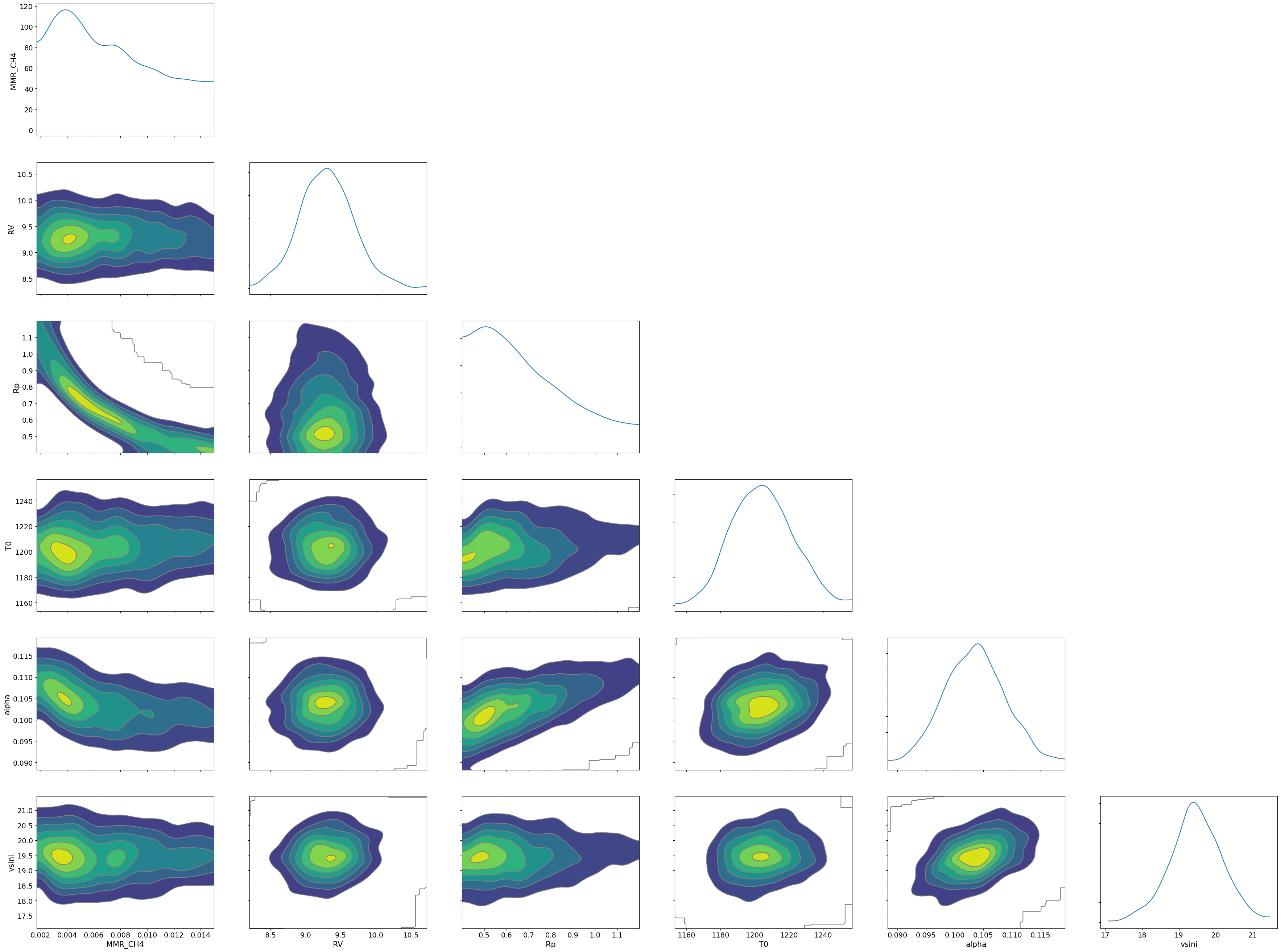
MMR_CH4 0.01 0.00 0.01 0.00 0.01 262.15 1.00
RV 9.30 0.38 9.30 8.65 9.91 608.21 1.00
Rp 0.68 0.20 0.64 0.40 0.99 267.23 1.00
T0 1204.59 17.39 1204.31 1179.03 1234.06 713.10 1.01
alpha 0.10 0.01 0.10 0.10 0.11 354.36 1.00
vsini 19.47 0.70 19.46 18.38 20.71 381.05 1.01
Number of divergences: 2
# SAMPLING
posterior_sample = mcmc.get_samples()
pred = Predictive(model_c, posterior_sample, return_sites=['y1'])
predictions = pred(rng_key_, y1=None)
median_mu1 = jnp.median(predictions['y1'], axis=0)
hpdi_mu1 = hpdi(predictions['y1'], 0.9)
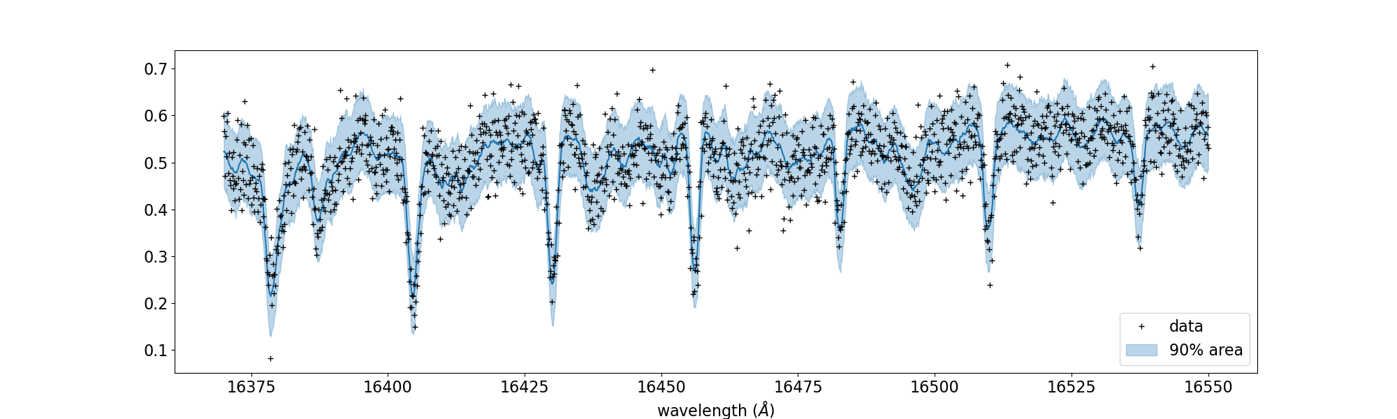
# PLOT
fig, ax = plt.subplots(nrows=1, ncols=1, figsize=(20, 6.0))
ax.plot(wavd[::-1], median_mu1, color='C0')
ax.plot(wavd[::-1], nflux, '+', color='black', label='data')
ax.fill_between(wavd[::-1],
                hpdi_mu1[0],
                hpdi_mu1[1],
                alpha=0.3,
                interpolate=True,
                color='C0',
                label='90% area')
plt.xlabel('wavelength ($\AA$)', fontsize=16)
plt.legend(fontsize=16)
plt.tick_params(labelsize=16)
plt.savefig("pred_diffmode" + str(diffmode) + ".png")
plt.close()
Draw a corner plot
pararr = ['Rp', 'T0', 'alpha', 'MMR_CH4', 'vsini', 'RV']
arviz.plot_pair(arviz.from_numpyro(mcmc),
                kind='kde',
                divergences=False,
                marginals=True)
plt.savefig("corner_diffmode" + str(diffmode) + ".png")
#plt.show()