SopPhoto: Computes Apparent Magnitude
Hajime Kawahara March 5th 2025
In ExoJAX, computed spectra can be easily converted into photometric
information, specifically apparent magnitude. This is achieved using
SopPhoto, one of the spectral operators. By default, the calculation
is performed using filter functions provided by
SVO. In this example, the
SDSS G-band filter is used.
from exojax.postproc.specop import SopPhoto

filter_name = "SLOAN/SDSS.g"
sop_photo = SopPhoto(filter_name, download=True)
/home/kawahara/anaconda3/lib/python3.10/site-packages/pandas/core/arrays/masked.py:60: UserWarning: Pandas requires version '1.3.6' or newer of 'bottleneck' (version '1.3.5' currently installed).
  from pandas.core import (
filter_id =  SLOAN/SDSS.g
You can check the available filters at http://svo2.cab.inta-csic.es/theory/fps/
resolution_photo= 6123.2
save  .database/filter/svo/SLOAN/SDSS.g.csv
save  .database/filter/svo/SLOAN/SDSS.g.info.csv
xsmode =  premodit
xsmode assumes ESLOG in wavenumber space: xsmode=premodit
Your wavelength grid is in *  descending  * order
The wavenumber grid is in ascending order by definition.
Please be careful when you use the wavelength grid.
/home/kawahara/exojax/src/exojax/utils.grids.py:82: UserWarning: Both input wavelength and output wavenumber are in ascending order.
  warnings.warn(
/home/kawahara/exojax/src/exojax/utils/grids.py:170: UserWarning: Resolution may be too small. R=6123.03886194115
  warnings.warn("Resolution may be too small. R=" + str(resolution), UserWarning)
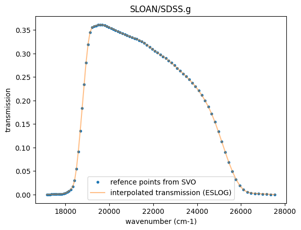
When SopPhoto is called, it calculates the transmission curve by
interpolating the transmission data obtained from SVO onto the
wavenumber grid in ESLOG base; nu_grid_filter,
transmission_filter. These interpolated transmissions can be
directly used for opa calculations. The resolution can be adjusted
by specifying the factor by which the original resolution is increased
using up_resolution_factor.
import matplotlib.pyplot as plt
plt.plot(sop_photo.nu_ref, sop_photo.transmission_ref, ".", label="refence points from SVO")
plt.plot(sop_photo.nu_grid_filter, sop_photo.transmission_filter, alpha=0.5,label="interpolated transmission (ESLOG)")
plt.legend()
plt.title(sop_photo.filter_id)
plt.xlabel("wavenumber (cm-1)")
plt.ylabel("transmission")
plt.show()
In this example, let’s compute the apparent magnitude (which is essentially the absolute magnitude!) of a blackbody sphere with the same temperature as the Sun placed at 10 pc.
Recall the flux from a black body sphere with a radius R, temperature T at distance of d is given by
\(f_\nu = \pi B_\nu (T) \frac{R^2}{d^2}\)
where \(B_\nu (T)\) is the Planck function.
# Sun
from exojax.rt.planck import piB
from exojax.utils.constants import RJ, Rs
from exojax.utils.constants import pc

flux = piB(5772.0, sop_photo.nu_grid_filter) * (Rs/RJ) ** 2 / (10.0) ** 2 * (RJ / pc)**2 #erg/s/cm2/cm-1

mag = sop_photo.apparent_magnitude(flux)
print(mag)
5.3326893