Simple Usage

1. Voigt profile

import numpy
import matplotlib.pyplot as plt
from exojax.spec import voigt

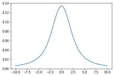
ExoJAX has both opacity calculators and radiative transfer algorithms. The basis of the former capacility is the Voigt function, which is the convolution of a Gaussian and a Lorentian.

x=numpy.linspace(-10,10,100)
y=voigt(x,1.0,2.0) #sigma_D=1.0, gamma_L=2.0
plt.plot(x,y)
plt.show()

2. Cross section

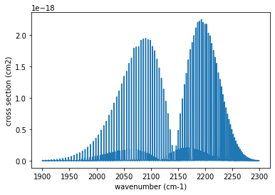
This software has many features, but the laziest use is to use spec.autospec. Let’s try to compute the cross section of carbon monooxide.

from exojax.spec.autospec import AutoXS

ExoJAX automatically downloads a molecular database, convert it to the feather format and save it in .database directory.

nus=numpy.linspace(1900.0,2300.0,40000,dtype=numpy.float64) #wavenumber (cm-1)
autoxs=AutoXS(nus,"ExoMol","CO") #using ExoMol CO (12C-16O). HITRAN and HITEMP are also supported.
xsv=autoxs.xsection(1000.0,1.0) #cross section for 1000K, 1bar (cm2)

Warning: CO is interpreted as 12C-16O
Recommendated database by ExoMol:  Li2015
CO/12C-16O/Li2015
broadf= True
Background atmosphere:  H2
Reading .database/CO/12C-16O/Li2015/12C-16O__Li2015.trans.bz2
.broad is used.
Broadening code level= a0
default broadening parameters are used for  71  J lower states in  152  states

0%|          | 0/19 [00:00<?, ?it/s]

# of lines= 3636
LPF selected

100%|██████████| 19/19 [00:01<00:00, 10.62it/s]

plt.plot(nus,xsv) #cm2
plt.xlabel("wavenumber (cm-1)")
plt.ylabel("cross section (cm2)")
plt.show()

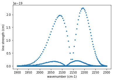
You can plot the line strengths.

ls=autoxs.linest(1000.0) #line strength for 1000K
plt.plot(autoxs.mdb.nu_lines,ls,".")
plt.xlabel("wavenumber (cm-1)")
plt.ylabel("line strength (cm)")
plt.show()

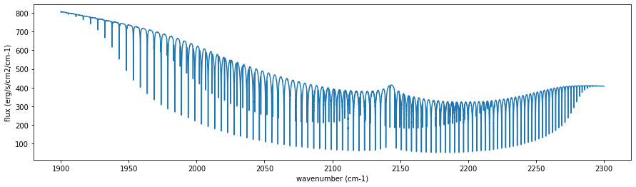
ExoJAX can solve the radiative transfer and derive the emission spectrum. Let’s try it using spec.autospec.AutRT

from exojax.utils.grids import wavenumber_grid
from exojax.spec.autospec import AutoRT

We need to assume a temperature-Pressure profile (T-P profile) to compute the emission spectrum. Here, we assume a power-law type T-P profile. In addition to CO, we assume H2-H2 and H2-He collisional induced absorption (CIA) as a continuum opacity.

nus,wav,res=wavenumber_grid(1900.0,2300.0,150000,"cm-1")
Parr=numpy.logspace(-8,2,100)
Tarr = 500.*(Parr/Parr[-1])**0.02
autort=AutoRT(nus,1.e5,2.33,Tarr,Parr) #g=1.e5 cm/s2, mmw=2.33
autort.addcia("H2-H2",0.74,0.74)       #CIA, mmr(H)=0.74
autort.addcia("H2-He",0.74,0.25)       #CIA, mmr(He)=0.25
autort.addmol("ExoMol","CO",0.01)      #CO line, mmr(CO)=0.01

xsmode assumes ESLOG in wavenumber space: mode=lpf
The wavenumber grid is evenly spaced in log space (ESLOG).
xsmode= auto
H2-H2
H2-He
Warning: CO is interpreted as 12C-16O
Recommendated database by ExoMol:  Li2015
CO/12C-16O/Li2015
broadf= True
Background atmosphere:  H2
Reading .database/CO/12C-16O/Li2015/12C-16O__Li2015.trans.bz2
.broad is used.
Broadening code level= a0
default broadening parameters are used for  71  J lower states in  152  states
# of lines 3636
# of lines= 3636
MODIT selected
xsmode= MODIT

/home/kawahara/exojax/src/exojax/spec/autospec.py:313: UserWarning: negative cross section detected #=3822040 fraction=0.2548026666666667
  warnings.warn(msg, UserWarning)

Let’s run the radiative transfer.

F=autort.rtrun()

fig=plt.figure(figsize=(15,4))
plt.plot(nus,F)
plt.xlabel("wavenumber (cm-1)")
plt.ylabel("flux (erg/s/cm2/cm-1)")
plt.show()

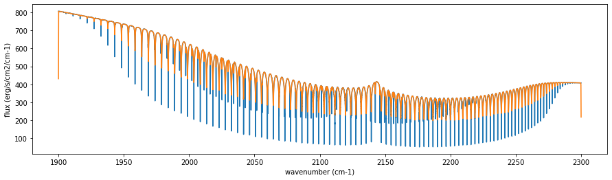
You may wanna take a planet spin rotation, RV shift, and observational sampling? Yes, we can.

nusobs=numpy.linspace(1900.0,2300.0,3000,dtype=numpy.float64) #observation wavenumber bin (cm-1)
Fobs=autort.spectrum(nusobs,100000.0,20.0,0.0) #R=100000, vsini=10km/s, RV=0km/s

This is just a convolution. So, you should ignore the edges.

fig=plt.figure(figsize=(15,4))
plt.plot(nus,F)
plt.plot(nusobs,Fobs)
plt.xlabel("wavenumber (cm-1)")
plt.ylabel("flux (erg/s/cm2/cm-1)")
plt.show()

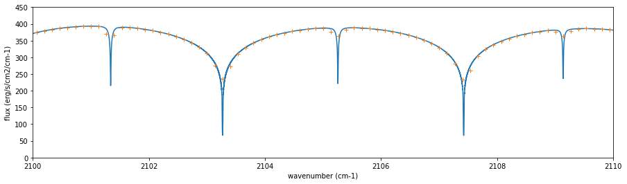
fig=plt.figure(figsize=(15,4))
plt.plot(nus,F)
plt.plot(nusobs,Fobs,"+")
plt.xlim(2100,2110)
plt.ylim(0,450)
plt.xlabel("wavenumber (cm-1)")
plt.ylabel("flux (erg/s/cm2/cm-1)")
plt.show()

Visualize the contribution function to see where the emission comes from.

from exojax.plot.atmplot import plotcf

cf=plotcf(nus,autort.dtau,Tarr,Parr,autort.dParr)

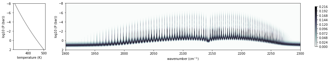
That’s it.