ExoMol, HITEMP, HITRAN
June 17th (2023) Hajime Kawahara, Yui Kawashima, Yui Kasagi
Since version 1.2, the standard molecular database I/O for ExoMol, HITEMP, and HITRAN was shared with the radis team. We moved the I/O for these database to exojax.spec.api.
ExoMol
How to load ExoMol CO database
>>> from exojax.spec.api import MdbExomol
>>> mdb = MdbExomol(".database/CO/12C-16O/Li2015", nurange=[4200.0, 4300.0])
We can check the attribute_names in mdb by
>>> attribute_names = [attr_name for attr_name, attr_value in mdb.__dict__.items() if not callable(attr_value) and not attr_name.startswith("__")]
>>> print(attribute_names)
['dbtype', 'path', 'exact_molecule_name', 'database', 'bkgdatm', 'Tref', 'gpu_transfer', 'Ttyp', 'broadf', 'simple_molecule_name', 'molmass', 'skip_optional_data', 'activation', 'name', 'molecule', 'local_databases', 'extra_params', 'downloadable', 'format', 'engine', 'tempdir', 'ds', 'verbose', 'parallel', 'nJobs', 'batch_size', 'minimum_nfiles', 'crit', 'margin', 'nurange', 'wmin', 'wmax', 'states_file', 'pf_file', 'def_file', 'broad_file', 'isotope_fullname', 'n_Texp_def', 'alpha_ref_def', 'gQT', 'T_gQT', 'QTref', 'trans_file', 'num_tag', 'elower_max', 'QTtyp', 'df_load_mask', 'A', 'nu_lines', 'elower', 'jlower', 'jupper', 'line_strength_ref', 'gpp', 'alpha_ref', 'n_Texp', 'gamma_natural', 'dev_nu_lines', 'logsij0']
Some opacity calculator (currently only PreMODIT) does not use some arrays on a GPU device. Switch gpu_transfer off in this case. Then, we can save the use of the device memory.
>>> mdb = MdbExomol(".database/CO/12C-16O/Li2015", nurange=[4200.0, 4300.0], gpu_transfer=False)
>>> mdb.logsij0
        Traceback (most recent call last):
         File "<stdin>", line 1, in <module>
         AttributeError: logsij0
This table is a short summary of the line information. “on” means gpu_transfer = True, off corresponds to False.
quantity |
instance |
unit |
off/on |
line center |
nu_lines |
cm-1 |
np/np |
lower state energy |
elower |
cm-1 |
np/jnp |
Einstein coefficient |
A |
s-1 |
np/jnp |
reference line strength |
line_strength_ref |
cm |
np/jnp |
log_e Sij0 |
logsij0 |
-/jnp |
|
statistical weight |
gupper |
np/jnp |
|
J_lower |
jlower |
np/jnp |
|
J_upper |
jupper |
np/jnp |
|
temperature exponent |
n_Tref |
np/jnp |
|
alpha_ref (gamma0) |
alpha_ref |
np/jnp |
|
natural broadening |
gamma_natural |
cm-1 |
np/jnp |
line center |
dev_nu_lines |
cm-1 |
-/jnp |
HITEMP
How to load HITEMP CO database
Here are examples for loading CO from HITEMP.
>>> from exojax.spec.api import MdbHitemp
>>> MdbHitemp("CO", nurange=[4200.0, 4300.0])
>>> MdbHitemp(".database/CO/", nurange=[4200.0, 4300.0])
>>> MdbHitemp(".database/05/", nurange=[4200.0, 4300.0])
The style used in ExoJAX 1 is also acceptable (not recommended):
>>> MdbHitemp(".database/CO/05_HITEMP2019/05_HITEMP2019.par.bz2", nurange=[4200.0, 4300.0])
If you have the error like,
Please fix/delete the radis.json entry, change the `databank_name`, or change the default local databases path entry 'DEFAULT_DOWNLOAD_PATH' in `radis.config` or ~/radis.json
remove radis.json and retry it.
quantity |
instance |
unit |
off/on |
line center |
nu_lines |
cm-1 |
np/np |
line center |
dev_nu_lines |
cm-1 |
-/jnp |
lower state energy |
elower |
cm-1 |
np/jnp |
natural broadening |
gamma_natural |
cm-1 |
np/jnp |
air pressure broadening |
gamma_air |
cm-1 |
np/jnp |
self broadning |
gamma_self |
cm-1 |
np/jnp |
Einstein coefficient |
A |
s-1 |
np/jnp |
reference line strength |
line_strength_ref |
cm |
np/jnp |
log_e Sij0 |
logsij0 |
-/jnp |
|
statistical weight |
gpp |
np/jnp |
|
temperature exponent |
n_air |
np/jnp |
Isotope
HITEMP includes all of the isotopes. To know which isotopes are included in mdb, use uniqiso instance.
>>> mdb = MdbHitemp(".database/CO/", nurange=[4200.0, 4210.0], crit=1.e-30)
>>> mdb.uniqiso #-> [1,2,3,4,6]
You can know what isotope name “isotope=1” corresponds to
>>> mdb.exact_isotope_name(1) #-> (12C)(16O)
Loading HITEMP for Each Isotope
Sometimes it’s useful to take it out for each isotope. To load C12 O16 (isotope = 1), use the isotope option. “isotope” is the isotope number used in HITRAN/HITEMP, which starts from 1.
>>> mdb = MdbHitemp(".database/CO/", nurange=[4200.0, 4300.0], isotope = 1)
Parition Function (Ratio) for Each Isotope
In MdbHitemp, QT_interp and qr_interp have the isotope option. Here is an example of specifying an isotope for the partition function computation.
>>> T = 1000 #K
>>> isotope = 1
>>> QT = mdb.QT_interp(isotope, T) # partition function Q(T) for isotope=1
>>> q_ratio = mdb.qr_interp(isotope, T) # partition function ratio Q(T)/Q(Tref)
Direct Load of the HITRAN parameter file (.par)
We can directly use the HITRAN parameter file (.par file). The following is an example of reading .par directly:
>>> from exojax.spec.api import MdbHitemp
>>> from exojax.utils.grids import wavenumber_grid
>>> nus, wav, res = wavenumber_grid(22920.0,23100.0,20000,unit="AA",xsmode="modit")
xsmode =  modit
xsmode assumes ESLOG in wavenumber space: mode=modit
>>> mdb = MdbHitemp("CO",nus,parfile="05_HITEMP_SAMPLE.par")
Optional Quantum States
As in the case of MdbExomol, we can use vibrational quantum numbers and electronic states for filtering See ” qstates ” for the use of the optional quantum states.
HITRAN
The mdb for HITRAN is currently functioning much almost the same as MdbHITEMP. However, due to the possibility of implementing different functions in the future, separate classes are provided.
How to load HITRAN CO database
>>> from exojax.spec.api import Mdbhitran
>>> Mdbhitran(".database/CO/", nurange=[4200.0, 4300.0])
>>> Mdbhitran(".database/05/", nurange=[4200.0, 4300.0])
The style used in ExoJAX 1 is also acceptable (not recommended):
>>> Mdbhitran(".database/CO/05_hit12.par", nurange=[4200.0, 4300.0])
Masking Line Information
We can mask the line information using “apply_mask_mdb” method. Here is an example:
>>> import numpy as np
>>> from exojax.utils.grids import wavenumber_grid
>>> from exojax.spec import api
>>> nus,wav,res=wavenumber_grid(6910,6990,100000,unit='cm-1',xsmode="premodit")
>>>
>>> # ExoMol
>>> mdb = api.MdbExomol("/home/kawashima/database/H2O/1H2-16O/POKAZATEL",nus)
>>> print(len(mdb.elower), np.min(mdb.elower))
>>>
>>> mask = mdb.elower > 100.
>>> mdb.apply_mask_mdb(mask)
>>> print(len(mdb.elower), np.min(mdb.elower))
>>>
>>> # HITEMP
>>> mdb = api.MdbHitemp("/home/kawashima/database/H2O/01_HITEMP2010",nus)
>>> print(len(mdb.n_air), np.min(mdb.n_air))
>>>
>>> mask = mdb.n_air > 0.01
>>> mdb.apply_mask_mdb(mask)
>>> print(len(mdb.n_air), np.min(mdb.n_air))
>>>
>>> # HITRAN
>>> mdb = api.MdbHitran("/home/kawashima/database/H2O/01_hit12.par",nus)
>>> print(len(mdb.n_air), np.min(mdb.n_air))
>>>
>>> mask = mdb.n_air > 0.01
>>> mdb.apply_mask_mdb(mask)
>>> print(len(mdb.n_air), np.min(mdb.n_air))
DataFrames
ExoJAX mdb class inherits DataFrame of the common API when calling “inherit_dataframe=True”, in “df” instance as. This DataFrame is not masked by “nurange” and/or “crit” options and has the format of Vaex lazy I/O.
>>> mdb = MdbExomol(".database/CO/12C-16O/Li2015", nurange=[4200.0, 4300.0], inherit_dataframe=True)
>>> mdb.df
#        i_upper    i_lower    A          nu_lines      gup    jlower    jupper    elower      Sij0
0        84         42         1.155e-06  2.405586      3      0         1         66960.7124  3.811968898414225e-164
1        83         41         1.161e-06  2.441775      3      0         1         65819.903   9.663028103692631e-162
2        82         40         1.162e-06  2.477774      3      0         1         64654.9206  2.7438392479197905e-159
3        81         39         1.159e-06  2.513606      3      0         1         63465.8042  8.73322833971394e-157
4        80         38         1.152e-06  2.549292      3      0         1         62252.5793  3.115220404216648e-154
...      ...        ...        ...        ...           ...    ...       ...       ...         ...
125,491  306        253        7.164e-10  22147.135424  15     6         7         80.7354     1.8282485593637477e-31
125,492  474        421        9.852e-10  22147.86595   23     10        11        211.4041    2.0425455665383687e-31
125,493  348        295        7.72e-10   22147.897299  17     7         8         107.6424    1.9589545250222689e-31
125,494  432        379        9.056e-10  22148.262711  21     9         10        172.978     2.0662209116961706e-31
125,495  390        337        8.348e-10  22148.273111  19     8         9         138.3903    2.0387827253771594e-31
For instance, if you want to call “i_upper”, use “values” like:
>>> i_upper = mdb.df.i_upper.values
>>> i_upper
array([ 84,  83,  82, ..., 348, 432, 390])
Notice the above array is not masked. So, the length is different from for instance “mdb.nu_lines”.
>>> len(i_upper)
125496
>>> len(mdb.nu_lines)
771
Quantum States Filtering (ExoMol/HITEMP)
You need an additional installation!!
Currently, we need develop branch of radis to use this capability (Sep 17/2023).
The only quantum state needed to calculate the cross section is the rotational number index. However, some databases also describe vibrational quantum numbers and electronic states. We can use this information to filter/mask.
If we want to filter the lines based on vibrational states (v) we can mask the lines with Data Frame.
To do this, we do not enable mdb during initialization. We also need to load the optional quantum states. Here is an example of the initialization.
>>> from exojax.utils.grids import wavenumber_grid
>>> from exojax.spec import api

>>> nus, wav, res = wavenumber_grid(24000.0, 26000.0, 1000, unit="AA")
>>> mdb = api.MdbExomol(""CO/12C-16O/Li2015/"", nus, optional_quantum_states=True, activation=False)
Then, let’s check DataFrame.
>>> print(mdb.df)
You find the following fields are available for Li2015:
i_upper i_lower A nu_lines gup jlower jupper elower v_l v_u kp_l kp_u Sij0
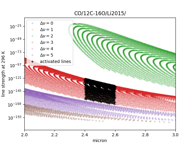
For instance, v_l means the rotational quantum number (nu) for the lower state, v_u the upper state. We would use the lines with the condition delta v = 3. Make the mask using DataFrame.
>>> mask = (mdb.df["v_u"] - mdb.df["v_l"] == 3)
Activate the mdb with the mask we made. The activation includes making the instances (such as mdb.nu_lines … ), computing broadening parameters etc.
>>> mdb.activate(mdb.df, mask)
Then, we can use mdb as usual. This is a plot of the activated lines and all of the lines in DataFrame.
See also ” Quatum states of Carbon Monoxide and Fortrat Diagram “
Masking Attributes
We can mask attributes even after activation. In the following example, we load “mdb” with activation (by default).
>>> import numpy as np
>>> from exojax.utils.grids import wavenumber_grid
>>> from exojax.spec import api
>>> nus,wav,res=wavenumber_grid(6910,6990,100000,unit='cm-1',xsmode="premodit")
xsmode =  premodit
xsmode assumes ESLOG in wavenumber space: mode=premodit
>>> mdb = api.MdbExomol(".database/H2O/1H2-16O/POKAZATEL",nus)
HITRAN exact name= H2(16O)
Background atmosphere:  H2
Reading .database/H2O/1H2-16O/POKAZATEL/1H2-16O__POKAZATEL__06900-07000.trans.bz2
.broad is used.
Broadening code level= a1
default broadening parameters are used for  12  J lower states in  63  states
>>> print(len(mdb.elower), np.min(mdb.elower))
26011826 23.794352
Then, we define a mask and apply it to mdb using apply_mask_mdb method.
>>> mask = mdb.elower > 100.
>>> mdb.apply_mask_mdb(mask)
>>> print(len(mdb.elower), np.min(mdb.elower))
26011817 134.90164
Uncertainty Code (HITEMP)
The with_error option makes the uncertainty code available for HITEMP (for HITRAN not yet; Issue398).
>>> lambda0 = 22920.0
>>> lambda1 = 23100.0
>>> nus, wav, res = wavenumber_grid(lambda0,
                                lambda1,
                                100000,
                                unit='AA',
                                xsmode="premodit")
>>> mdb = api.MdbHitemp("CO",nus, with_error=True)
>>> mdb.ierr
mdb.ierr contains the sets of the uncertainty code , but it’s not user-friendy. Use mdb.add_error() to generate more user-friendly attributes.
>>> mdb.add_error()
>>> mdb.nu_lines_err
array([4, 3, 3, 3, 4, 3, 4, 3, 3, 3, 3, 4, 4, 3, 3, 4, 4, 3, 4, 3, 4, 3,
   4, 4, 3, 4, 3, 3, 3, 4, 3, 3, 3, 4, 3, 3, 4, 3, 3, 3, 4, 3, 3, 4,
   3, 3, 3, 3, 3, 3, 4, 3, 3, 3, 4, 3, 3, 3, 3, 3, 4, 3, 3, 3, 3, 3,
   3, 3, 3, 4, 3, 3, 3, 4, 3, 4, 4, 3, 3, 3, 3, 3, 3, 3, 4, 3, 3, 4,
   3, 3, 3, 3, 3, 3, 4, 3, 3, 3, 3, 3, 4, 3, 3, 3, 3, 3, 4, 3, 3, 3,
   3, 3, 4, 3, 3, 3, 3, 4, 3, 3, 3, 3, 3, 4, 4, 3, 4, 3, 3, 3, 3, 3,
   3, 3, 3, 4, 3, 4, 3, 3, 3, 3, 3, 3, 3, 3, 3, 3, 4, 3, 4, 3, 3, 4,
   3, 4, 3, 3, 3, 3, 4, 3, 3, 3, 3, 4, 3, 3, 3, 4, 3, 4, 3, 3, 3, 3,
   3, 4, 3, 3, 3, 3, 3, 3, 3, 4, 4, 3, 3, 4, 3, 4, 3, 3, 3, 3, 3, 4,
   4, 3, 3, 3, 3, 3, 3, 4, 3, 3, 3, 4, 3, 3, 3, 4, 3, 3, 3, 3, 3, 3,
   4, 4, 3, 3, 4, 3, 3, 3, 4, 3, 4, 3, 4, 4, 3, 4, 3, 3, 3, 3, 3, 3,
   3, 3, 3, 3, 3, 3, 3, 3, 3, 3, 3, 3, 3, 3, 3, 3, 4, 4])
This makes the attributes nu_lines_err, line_strength_ref_err, gamma_air_err, gamma_self_err, n_air_err,and delta_air_err availbale. These quantities provide the uncertainty code for nu_lines, line_strength_ref, gamma_air, gamma_self, n_air,and delta_air, respectively.