Fitting a spectrum model using Gradient Descent Based Optimization.

last update: July 2nd Hajime Kawahara

The ability of the gradient-based optimizations is s one of the major advantages of ExoJAX. Here we demonstrate how to optimize the model using jaxopt package.

import pandas as pd
import numpy as np
import matplotlib.pyplot as plt
import jax.numpy as jnp

Use 64-bit.

from jax.config import config

config.update("jax_enable_x64", True)

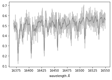
Here, we use a mock CH4 spectrum precomputed by ExoJAX. Also, we normalize it and add some noise.

import pkg_resources
from exojax.spec.unitconvert import nu2wav
from exojax.test.data import SAMPLE_SPECTRA_CH4_NEW

# loading the data
filename = pkg_resources.resource_filename(
    'exojax', 'data/testdata/' + SAMPLE_SPECTRA_CH4_NEW)
dat = pd.read_csv(filename, delimiter=",", names=("wavenumber", "flux"))
nusd = dat['wavenumber'].values
flux = dat['flux'].values
wavd = nu2wav(nusd)

sigmain = 0.05
norm = 20000
nflux = flux / norm + np.random.normal(0, sigmain, len(wavd))


plt.plot(wavd[::-1],nflux,alpha=0.5,color="gray")
plt.plot(wavd[::-1],flux/norm,alpha=1,color="gray")

plt.xlabel("wavelength $\AA$")
plt.show()

Let’s make a model, which should be include CH4, CIA (H2-H2), spin rotation, and response… So, import everthing we need. We use PreMODIT as opa.

from exojax.utils.grids import wavenumber_grid
from exojax.spec.atmrt import ArtEmisPure
from exojax.spec.api import MdbExomol
from exojax.spec.opacalc import OpaPremodit
from exojax.spec.contdb import CdbCIA
from exojax.spec.opacont import OpaCIA
from exojax.spec.specop import SopRotation
from exojax.spec.specop import SopInstProfile
from exojax.utils.instfunc import resolution_to_gaussian_std

/home/kawahara/exojax/src/exojax/spec/dtau_mmwl.py:14: FutureWarning: dtau_mmwl might be removed in future.
  warnings.warn("dtau_mmwl might be removed in future.", FutureWarning)

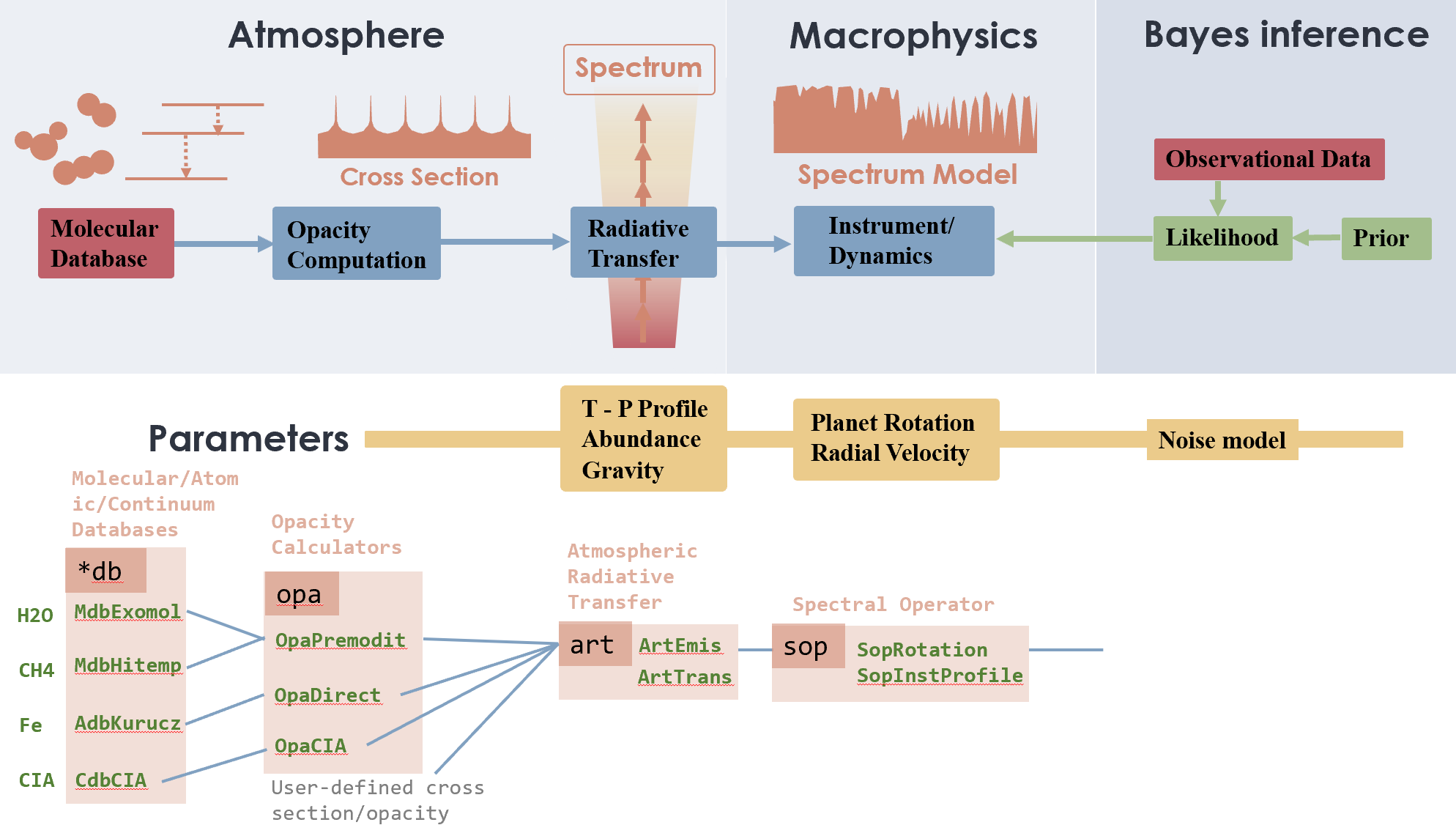
Again recall this figure.

from IPython.display import Image
Image("../exojax.png")

Here we will infer here Rp, RV, MMR_CO, T0, alpha, and Vsini.

First, set the model wavenumber grids, which should cover the observational range, and the instrumental setting, and Atmospheric RT (layer) setting, art.

Nx = 1500
nu_grid, wav, res = wavenumber_grid(np.min(wavd) - 5.0,
                                np.max(wavd) + 5.0,
                                Nx,
                                unit="AA",
                                xsmode="premodit")

#Atmospheric setting by "art"
Tlow = 400.0
Thigh = 1500.0
art = ArtEmisPure(nu_grid, pressure_top=1.e-8, pressure_btm=1.e2, nlayer=100)
art.change_temperature_range(Tlow, Thigh)
Mp = 33.2

#instrumental setting
Rinst = 100000.
beta_inst = resolution_to_gaussian_std(Rinst)

xsmode =  premodit
xsmode assumes ESLOG in wavenumber space: mode=premodit

/home/kawahara/exojax/src/exojax/utils/grids.py:126: UserWarning: Resolution may be too small. R=129859.29489937567
  warnings.warn('Resolution may be too small. R=' + str(resolution),

Loading the databases, mdb for ExoMol/CH4 and cdb for CIA. Also, define opa for both databases. It takes ~ a few minites to initialize OpaPremodit (if you do not have the database, it takes more for downloading for the first time). Have a coffee and wait.

### CH4 setting (PREMODIT)
mdb = MdbExomol('.database/CH4/12C-1H4/YT10to10/',
                nurange=nu_grid,
                gpu_transfer=False)
print('N=', len(mdb.nu_lines))
diffmode = 0
opa = OpaPremodit(mdb=mdb,
                  nu_grid=nu_grid,
                  diffmode=diffmode,
                  auto_trange=[Tlow, Thigh],
                  dit_grid_resolution=0.2)

## CIA setting
from exojax.spec import molinfo

cdbH2H2 = CdbCIA('.database/H2-H2_2011.cia', nu_grid)
opcia = OpaCIA(cdb=cdbH2H2, nu_grid=nu_grid)
mmw = 2.33  # mean molecular weight
mmrH2 = 0.74
molmassH2 = molinfo.molmass_isotope('H2')
vmrH2 = (mmrH2 * mmw / molmassH2)  # VMR

/home/kawahara/exojax/src/exojax/utils/molname.py:133: FutureWarning: e2s will be replaced to exact_molname_exomol_to_simple_molname.
  warnings.warn(
/home/kawahara/exojax/src/exojax/utils/molname.py:49: UserWarning: No isotope number identified.
  warnings.warn("No isotope number identified.",UserWarning)
/home/kawahara/exojax/src/exojax/utils/molname.py:49: UserWarning: No isotope number identified.
  warnings.warn("No isotope number identified.",UserWarning)
/home/kawahara/exojax/src/exojax/spec/molinfo.py:28: UserWarning: exact molecule name is not Exomol nor HITRAN form.
  warnings.warn("exact molecule name is not Exomol nor HITRAN form.")
/home/kawahara/exojax/src/exojax/spec/molinfo.py:29: UserWarning: No molmass available
  warnings.warn("No molmass available", UserWarning)

HITRAN exact name= (12C)(1H)4
HITRAN exact name= (12C)(1H)4
Background atmosphere:  H2
Reading .database/CH4/12C-1H4/YT10to10/12C-1H4__YT10to10__06000-06100.trans.bz2
Reading .database/CH4/12C-1H4/YT10to10/12C-1H4__YT10to10__06100-06200.trans.bz2
.broad is used.
Broadening code level= a1
default broadening parameters are used for  23  J lower states in  40  states
N= 76483758
OpaPremodit: params automatically set.
Robust range: 397.77407283130566 - 1689.7679243628259 K
Tref changed: 296.0K->1153.6267095763965K
Tref_broadening is set to  774.5966692414833 K
# of reference width grid :  3
# of temperature exponent grid : 2

uniqidx: 100%|██████████| 2/2 [00:03<00:00,  1.67s/it]

Premodit: Twt= 461.3329793405918 K Tref= 1153.6267095763965 K
Making LSD:|####################| 100%
H2-H2

We have only 76,483,758 CH4 lines.

print(len(mdb.nu_lines))

76483758

Setting spectral operators.

from exojax.utils.astrofunc import gravity_jupiter
sop_rot = SopRotation(nu_grid,res,vsini_max=100.0)
sop_inst = SopInstProfile(nu_grid,res,vrmax=100.0)

/home/kawahara/exojax/src/exojax/utils/grids.py:126: UserWarning: Resolution may be too small. R=129859.29489937567
  warnings.warn('Resolution may be too small. R=' + str(resolution),
/home/kawahara/exojax/src/exojax/utils/grids.py:126: UserWarning: Resolution may be too small. R=129859.29489937567
  warnings.warn('Resolution may be too small. R=' + str(resolution),

Now we write the model, which is used in HMC-NUTS.

#response and rotation settings


def model_c(params,boost):
    Rp,RV,MMR_CH4,T0,alpha,vsini,RV=params*boost

    Tarr = art.powerlaw_temperature(T0, alpha)
    g = gravity_jupiter(Rp=Rp, Mp=Mp)  # gravity in the unit of Jupiter
    #molecule
    xsmatrix = opa.xsmatrix(Tarr, art.pressure)
    mmr_arr = art.constant_mmr_profile(MMR_CH4)
    dtaumCH4 = art.opacity_profile_lines(xsmatrix, mmr_arr, opa.mdb.molmass, g)
    #continuum
    logacia_matrix = opcia.logacia_matrix(Tarr)
    dtaucH2H2 = art.opacity_profile_cia(logacia_matrix, Tarr, vmrH2, vmrH2,
                                        mmw, g)
    #total tau
    dtau = dtaumCH4 + dtaucH2H2
    F0 = art.run(dtau, Tarr) / norm
    Frot = sop_rot.rigid_rotation(F0, vsini, u1=0.0, u2=0.0)
    Frot_inst = sop_inst.ipgauss(Frot, beta_inst)
    mu = sop_inst.sampling(Frot_inst, RV, nusd)
    return mu

Here, we use JAXopt as an optimizer. JAXopt is not automatically installed. If you need install it by pip:

pip install jaxopt

import jaxopt

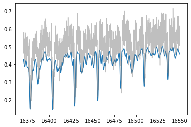
We use a GradientDescent as an optimizer. Let’s normalize the parameters.

#Rp,RV,MMR_CH4,T0,alpha,vsini, RV
boost=np.array([1.0,10.0,0.1,1000.0,1.e-3,10.0,10.0])
initpar=np.array([0.8,9.0,0.01,1200.0,0.1,17.0,0.0])/boost

f = model_c(initpar,boost)
plt.plot(wavd[::-1],f)
plt.plot(wavd[::-1],nflux,alpha=0.5,color="gray")

[<matplotlib.lines.Line2D at 0x7f234d98e0d0>]

Define the objective function by a L2 norm.

def objective(params):
    f=nflux-model_c(params,boost)
    g=jnp.dot(f,f)
    return g

Then, run the gradient descent.

gd = jaxopt.GradientDescent(fun=objective, maxiter=1000, stepsize=1.e-4)
res = gd.run(init_params=initpar)
params, state = res

The best-fit parameters

params*boost

DeviceArray([3.32046971e+00, 9.00000000e+00, 1.25542304e-01,
             2.10939481e+03, 1.00095859e-01, 1.93251005e+01,
             1.14472806e+01], dtype=float64)

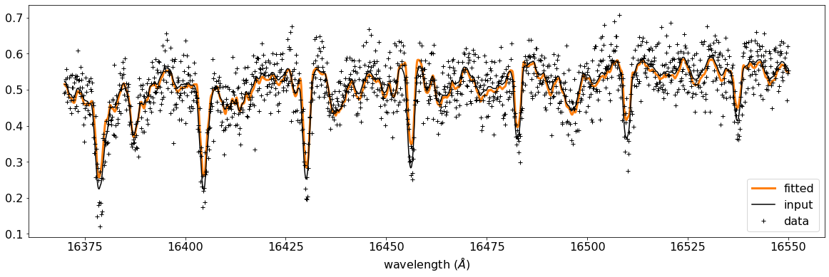
Plot the results. Good but a bit poor compared with the input… O.K. I prefer ADAM to GD let’s try next.

model=model_c(params,boost)
inmodel=model_c(initpar,boost)
fig, ax = plt.subplots(nrows=1, ncols=1, figsize=(20,6.0))
ax.plot(wavd[::-1],model,color="C1",lw=3,label="fitted")
ax.plot(wavd[::-1],flux/norm,alpha=1,color="black",label="input")

#ax.plot(wavd[::-1],inmodel,color="gray",lw=3,label="initial parameter")
ax.plot(wavd[::-1],nflux,"+",color="black",label="data")
plt.xlabel("wavelength ($\AA$)",fontsize=16)
plt.legend(fontsize=16)
plt.tick_params(labelsize=16)
plt.savefig("gradient_descent_jaxopt.png")

BTW, We can do the optimization one by one update. It’s useful when you wanna visualize the optimization process.

import tqdm
gd = jaxopt.GradientDescent(fun=objective, stepsize=1.e-4)
state = gd.init_state(initpar)
params=np.copy(initpar)

params_gd=[]
Nit=300
for _ in  tqdm.tqdm(range(Nit)):
    params,state=gd.update(params,state)
    params_gd.append(params)

100%|██████████| 300/300 [00:40<00:00,  7.41it/s]

Using ADAM optimizer

You might use ADAM, instead of a simple GD. Yes, you can.

from jaxopt import OptaxSolver
import optax

import tqdm
adam = OptaxSolver(opt=optax.adam(2.e-2), fun=objective)
state = adam.init_state(initpar)
params_a=np.copy(initpar)

params_adam=[]
Nit=300
for _ in  tqdm.tqdm(range(Nit)):
    params_a,state=adam.update(params_a,state)
    params_adam.append(params_a)

100%|██████████| 300/300 [00:20<00:00, 14.31it/s]

model_adam=model_c(params_a,boost)
fig, ax = plt.subplots(nrows=1, ncols=1, figsize=(20,6.0))
ax.plot(wavd[::-1],model,color="C1",lw=4,label="GD")
ax.plot(wavd[::-1],model_adam,color="C2",lw=4,ls="dashed",label="ADAM")
ax.plot(wavd[::-1],flux/norm,alpha=1,color="black",label="input")

#ax.plot(wavd[::-1],inmodel,color="gray",lw=3,label="initial parameter")
ax.plot(wavd[::-1],nflux,"+",color="black",label="data")
plt.xlabel("wavelength ($\AA$)",fontsize=16)
plt.legend(fontsize=16)
plt.tick_params(labelsize=16)
plt.savefig("gradient_descent_jaxopt.png")

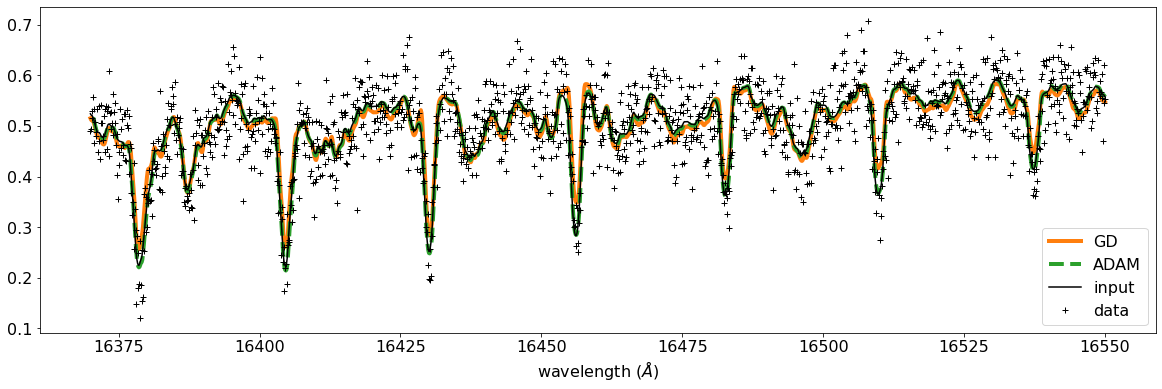
ADAM is faster and better than GD? I love ADAM.

# if you wanna optimize at once, run the following:
# res = solver.run(init_params=initpar)
# params, state = res

make a movie

Make the movie directory (mkdir movie), and let’s make squential png files.

inmodel=model_c(initpar,boost)
for i in tqdm.tqdm(range(Nit)):
    spec_gd=model_c(params_gd[i],boost)
    spec_adam=model_c(params_adam[i],boost)
    fig, ax = plt.subplots(nrows=1, ncols=1, figsize=(20,6.0))
    ax.plot(wavd[::-1],spec_gd,color="C0",lw=3,label="GD")
    ax.plot(wavd[::-1],spec_adam,color="C1",lw=3,label="ADAM")
    ax.plot(wavd[::-1],inmodel,color="gray",label="initial parameter")
    ax.plot(wavd[::-1],nflux,"+",color="black",label="data")
    plt.xlabel("wavelength ($\AA$)",fontsize=16)
    plt.tick_params(labelsize=16)
    plt.ylim(0.0,0.6)
    plt.legend(loc="lower left",fontsize=14)
    plt.savefig("movie/gradient_descent_jaxopt"+str(i).zfill(4)+".png")
    plt.close()

100%|██████████| 300/300 [00:57<00:00,  5.19it/s]

#for instance, make a movie by
# > ffmpeg -r 30 -i gradient_descent_jaxopt%04d.png -vcodec libx264 -pix_fmt yuv420p -r 60 outx.mp4