Ackerman and Marley Cloud Model
Here, we try to compute a cloud opacity using Ackerman and Marley Model. We consider enstatite (MgSiO3) and Fe clouds.
import jax.numpy as jnp
import matplotlib.pyplot as plt
import numpy as np
Setting a simple atmopheric model. We need the density of atmosphere.
from exojax.spec import rtransfer as rt
from exojax.utils.constants import kB, m_u

NP = 100
Parr, dParr, k = rt.pressure_layer(NP=NP, logPtop=-8., logPbtm=4.0)
alpha = 0.097
T0 = 1200.
Tarr = T0 * (Parr)**alpha

mu = 2.0  # mean molecular weight
R = kB / (mu * m_u)
rho = Parr / (R * Tarr)
The solar abundance can be obtained using utils.zsol.nsol. Here, we assume a maximum VMR for MgSiO3 and Fe from solar abundance.
from exojax.utils.zsol import nsol

n = nsol()  #solar abundance
VMR_enstatite = np.min([n["Mg"], n["Si"], n["O"] / 3])
VMR_Fe = n["Fe"]
Vapor saturation pressures can be obtained using atm.psat
from exojax.atm.psat import Psat_enstatite_AM01, Psat_Fe_solid

P_enstatite = Psat_enstatite_AM01(Tarr)
P_fe_sol = Psat_Fe_solid(Tarr)
Compute a cloud base pressure.
from exojax.atm.amclouds import get_Pbase

Pbase_enstatite = get_Pbase(Parr, P_enstatite, VMR_enstatite)
Pbase_Fe_sol = get_Pbase(Parr, P_fe_sol, VMR_Fe)
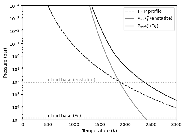
The cloud base is located at the intersection of a TP profile and the vapor saturation puressure devided by VMR.
plt.plot(Tarr, Parr, color="black", ls="dashed", label="T - P profile")
plt.plot(Tarr,
         P_enstatite / VMR_enstatite,
         label="$P_{sat}/\\xi$ (enstatite)",
         color="gray")
plt.axhline(Pbase_enstatite, color="gray", alpha=0.7, ls="dotted")
plt.text(500, Pbase_enstatite * 0.8, "cloud base (enstatite)", color="gray")

plt.plot(Tarr, P_fe_sol / VMR_Fe, label="$P_{sat}/\\xi$ (Fe)", color="black")
plt.axhline(Pbase_Fe_sol, color="black", alpha=0.7, ls="dotted")
plt.text(500, Pbase_Fe_sol * 0.8, "cloud base (Fe)", color="black")

plt.yscale("log")
plt.ylim(1.e-7, 10000)
plt.xlim(0, 2700)
plt.gca().invert_yaxis()
plt.legend()
plt.xlabel("Temperature (K)")
plt.ylabel("Pressure (bar)")
plt.savefig("pbase.pdf", bbox_inches="tight", pad_inches=0.0)
plt.savefig("pbase.png", bbox_inches="tight", pad_inches=0.0)
plt.show()
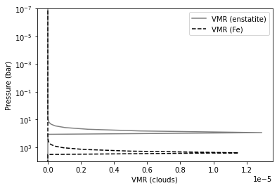
Compute VMRs of clouds. Because Parr is an array, we apply jax.vmap to atm.amclouds.VMRclouds.
from jax import vmap
from exojax.atm.amclouds import VMRcloud

get_VMRc = vmap(VMRcloud, (0, None, None, None), 0)

fsed = 3
VMRbase_enstatite = VMR_enstatite
VMRc_enstatite = get_VMRc(Parr, Pbase_enstatite, fsed, VMR_enstatite)

VMRbase_Fe = VMR_Fe
VMRc_Fe = get_VMRc(Parr, Pbase_Fe_sol, fsed, VMR_Fe)
Here is the VMR distribution.
plt.figure()
plt.gca().get_xaxis().get_major_formatter().set_powerlimits([-3, 3])
plt.plot(VMRc_enstatite, Parr, color="gray", label="VMR (enstatite)")
plt.plot(VMRc_Fe, Parr, color="black", ls="dashed", label="VMR (Fe)")

plt.yscale("log")
plt.ylim(1.e-7, 10000)
plt.gca().invert_yaxis()
plt.legend()
plt.xlabel("VMR (clouds)")
plt.ylabel("Pressure (bar)")
plt.savefig("vmrcloud.pdf", bbox_inches="tight", pad_inches=0.0)
plt.savefig("vmrcloud.png", bbox_inches="tight", pad_inches=0.0)
plt.show()
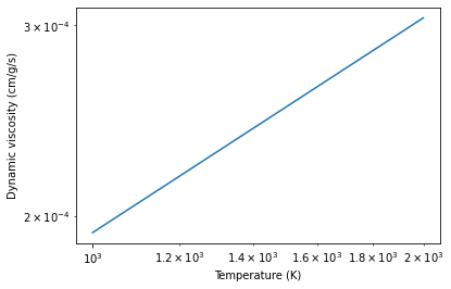
Compute dynamic viscosity in H2 atmosphere (cm/g/s)
from exojax.atm.viscosity import eta_Rosner, calc_vfactor

T = np.logspace(np.log10(1000), np.log10(2000))
vfactor, Tr = calc_vfactor("H2")
eta = eta_Rosner(T, vfactor)
plt.plot(T, eta)
plt.xscale("log")
plt.yscale("log")
plt.xlabel("Temperature (K)")
plt.ylabel("Dynamic viscosity (cm/g/s)")
plt.show()
The pressure scale height can be computed using atm.atmprof.Hatm.
from exojax.atm.atmprof import Hatm

T = 1000  #K
mu = 2  #mean molecular weight
print("scale height=", Hatm(1.e5, T, mu), "cm")
scale height= 415722.9931793715 cm
We need a density of condensates.
rhoc_enstatite = 3.192  #g/cm3 Lodders and Fegley (1998)
rhoc_Fe = 7.875

from exojax.spec.molinfo import molmass

mu = molmass("H2")
muc_enstatite = molmass("MgSiO3")
muc_Fe = molmass("Fe")
Let’s compute the terminal velocity. We can compute the terminal velocity of cloud particle using atm.vterm.vf. vmap is again applied to vf.
from exojax.atm.viscosity import calc_vfactor, eta_Rosner
from exojax.atm.vterm import vf
from jax import vmap

vfactor, trange = calc_vfactor(atm="H2")
rarr = jnp.logspace(-6, -4, 2000)  #cm
drho = rhoc_enstatite - rho
eta_fid = eta_Rosner(Tarr, vfactor)

g = 1.e5
vf_vmap = vmap(vf, (None, None, 0, 0, 0))
vfs = vf_vmap(rarr, g, eta_fid, drho, rho)
Kzz/L will be used to calibrate \(r_w\). following Ackerman and Marley 2001
Kzz = 1.e5  #cm2/s
sigmag = 2.0
alphav = 1.3
L = Hatm(g, 1500, mu)
Kzz/L
0.16163647693888086
for i in range(0, len(Tarr)):
    plt.plot(rarr, vfs[i, :], alpha=0.2, color="gray")
plt.xscale("log")
plt.yscale("log")
plt.axhline(Kzz / L, label="Kzz/H", color="C2", ls="dotted")
plt.ylabel("stokes terminal velocity (cm/s)")
plt.xlabel("condensate size (cm)")
Text(0.5, 0, 'condensate size (cm)')
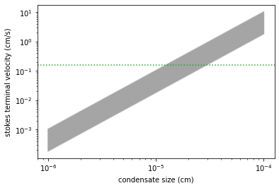
Find the intersection.
from exojax.atm.amclouds import find_rw

vfind_rw = vmap(find_rw, (None, 0, None), 0)
rw = vfind_rw(rarr, vfs, Kzz / L)
Then, \(r_g\) can be computed from \(r_w\) and other quantities.
from exojax.atm.amclouds import get_rg

rg = get_rg(rw, fsed, alphav, sigmag)
plt.plot(rg * 1.e4, Parr, label="$r=r_g$", color="black")
plt.plot(rw * 1.e4, Parr, ls="dashed", label="$r=r_w$", color="black")
plt.ylim(1.e-7, 10000)
plt.xlabel("$r$ (micron)")
plt.ylabel("Pressure (bar)")
plt.yscale("log")
plt.savefig("rgrw.png")
plt.legend()
<matplotlib.legend.Legend at 0x7ff18c758250>
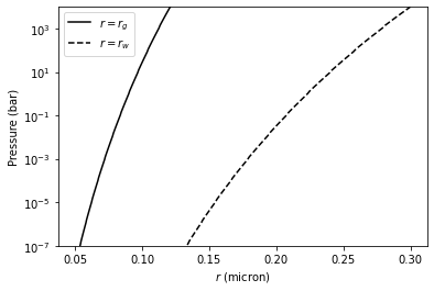
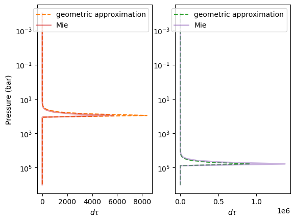
We found here the particle size is basically sub-micron. So, we should use the Rayleigh scattering. But, here, we try to use the geometric cross section instead though this is wrong.
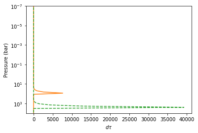
from exojax.atm.amclouds import dtau_cloudgeo

dtau_enstatite = dtau_cloudgeo(Parr, muc_enstatite, rhoc_enstatite, mu,
                               VMRc_enstatite, rg, sigmag, g)
dtau_Fe = dtau_cloudgeo(Parr, muc_Fe, rhoc_Fe, mu, VMRc_Fe, rg, sigmag, g)
plt.plot(dtau_enstatite, Parr, color="C1")
plt.plot(dtau_Fe, Parr, color="C2", ls="dashed")
plt.yscale("log")
plt.ylim(1.e-7, 10000)
plt.xlabel("$d\\tau$")
plt.ylabel("Pressure (bar)")
#plt.xscale("log")
plt.gca().invert_yaxis()
Let’s compare with CIA
#CIA
from exojax.utils.grids import wavenumber_grid

nus, wav, res = wavenumber_grid(9500, 30000, 1000, unit="AA")

from exojax.spec import contdb

cdbH2H2 = contdb.CdbCIA('.database/H2-H2_2011.cia', nus)
xsmode assumes ESLOG in wavenumber space: mode=lpf
H2-H2
/home/kawahara/exojax/src/exojax/utils/grids.py:123: UserWarning: Resolution may be too small. R=868.7669794117727
  warnings.warn('Resolution may be too small. R=' + str(resolution),
from exojax.spec.rtransfer import dtauCIA

mmw = 2.33  #mean molecular weight
mmrH2 = 0.74
molmassH2 = molmass("H2")
vmrH2 = (mmrH2 * mmw / molmassH2)  #VMR
dtaucH2H2=dtauCIA(nus,Tarr,Parr,dParr,vmrH2,vmrH2,\
            mmw,g,cdbH2H2.nucia,cdbH2H2.tcia,cdbH2H2.logac)
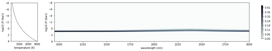
dtau = dtaucH2H2 + dtau_enstatite[:, None] + dtau_Fe[:, None]
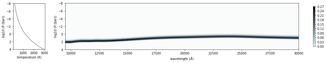
from exojax.plot.atmplot import plotcf

plotcf(nus, dtau, Tarr, Parr, dParr, unit="nm")
plt.show()
from exojax.plot.atmplot import plotcf

plotcf(nus, dtaucH2H2, Tarr, Parr, dParr, unit="AA")
plt.show()
from exojax.plot.atmplot import plotcf

plotcf(nus,
       dtau_enstatite[:, None] + np.zeros_like(dtaucH2H2),
       Tarr,
       Parr,
       dParr,
       unit="AA")
plt.show()
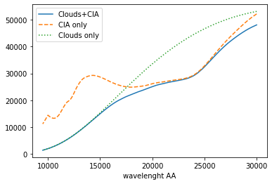
from exojax.spec import planck
from exojax.spec.rtransfer import rtrun

sourcef = planck.piBarr(Tarr, nus)
F0 = rtrun(dtau, sourcef)
F0CIA = rtrun(dtaucH2H2, sourcef)
F0cl = rtrun(dtau_enstatite[:, None] + np.zeros_like(dtaucH2H2), sourcef)
plt.plot(wav[::-1], F0, label="Clouds+CIA")
plt.plot(wav[::-1], F0CIA, label="CIA only", ls="dashed")
plt.plot(wav[::-1], F0cl, label="Clouds only", ls="dotted")
plt.xlabel("wavelenght AA")
plt.legend()
plt.show()